A Comprehensive Computational Pipeline for Stem Cell scRNA-seq Data: From Foundational Analysis to Clinical Translation
This article provides a detailed guide to the computational analysis of single-cell RNA sequencing (scRNA-seq) data from stem cell research.
A Comprehensive Computational Pipeline for Stem Cell scRNA-seq Data: From Foundational Analysis to Clinical Translation
Abstract
This article provides a detailed guide to the computational analysis of single-cell RNA sequencing (scRNA-seq) data from stem cell research. Aimed at researchers, scientists, and drug development professionals, it covers the foundational principles of scRNA-seq, including cell sorting and quality control for sensitive stem cell populations. It explores a complete methodological workflow from data pre-processing and integration to clustering, annotation, and trajectory inference. The guide further addresses critical troubleshooting and optimization strategies, such as feature selection for improved data integration. Finally, it discusses validation techniques and the comparative performance of analysis tools, concluding with the translational potential of these pipelines in advancing regenerative medicine and therapeutic discovery.
Laying the Groundwork: Core Principles and Experimental Design for Stem Cell scRNA-seq
Single-cell RNA sequencing (scRNA-seq) represents a revolutionary advance in transcriptomic analysis, enabling researchers to profile gene expression at the level of individual cells rather than population averages [1] [2]. This technological breakthrough has proven particularly valuable in stem cell research, where cellular heterogeneity plays a crucial role in fate decisions, differentiation potential, and therapeutic applications [1]. Even in seemingly homogeneous pluripotent stem cell cultures, scRNA-seq has revealed distinct subpopulations of cells in different functional states, challenging previous assumptions about uniform cell populations and providing unprecedented insights into the complexity of stem cell biology [3].
Traditional bulk RNA sequencing approaches obscure cell-to-cell variation by measuring average expression across thousands of cells, effectively masking rare cell types and continuous transitional states [1] [2]. In contrast, scRNA-seq captures this heterogeneity, allowing identification of novel cell subtypes, reconstruction of developmental trajectories, and discovery of regulatory networks governing cell fate decisions [1]. For stem cell researchers, this capability has transformed our understanding of pluripotency, lineage commitment, and the molecular mechanisms underlying self-renewal and differentiation.
Key scRNA-seq Technologies and Methodologies
The complete scRNA-seq workflow encompasses multiple critical steps from sample preparation to data generation, each requiring careful optimization for stem cell applications.
Single-Cell Isolation Methods
The first critical step in any scRNA-seq experiment involves isolating viable single cells from culture or tissue. The choice of isolation method significantly impacts throughput, viability, and experimental outcomes.
- Microwell-based platforms: Technologies like Fluidigm C1 provide automated single-cell lysis, RNA extraction, and cDNA synthesis with visual inspection capability, though with limited throughput [4] [2]. These systems allow researchers to exclude empty wells or those containing damaged cells prior to library preparation, improving data quality.
- Droplet-based methods: Commercial platforms like 10x Genomics Chromium system use microfluidics to encapsulate individual cells with barcoded beads in nanoliter droplets, enabling high-throughput profiling of thousands to millions of cells [4] [5]. This approach dramatically reduces reagent costs and processing time but offers less control over cell input.
- Fluorescence-Activated Cell Sorting (FACS): This remains the gold standard for isolating specific cell populations based on surface markers, making it ideal for studying rare stem cell subtypes [2]. FACS provides high purification efficiency and the ability to select cells based on multiple fluorescent parameters simultaneously.
Library Preparation Protocols
scRNA-seq protocols diverge primarily in their approach to cDNA synthesis and amplification, with significant implications for data quality and applications.
- Full-length transcript protocols: Methods like Smart-seq2 generate sequencing libraries with uniform coverage across entire transcripts, enabling detection of alternative splicing, allele-specific expression, and single-nucleotide polymorphisms [6] [5]. These protocols are ideal for detailed characterization of transcriptional heterogeneity in stem cell populations.
- 3' or 5' end-counting methods: Droplet-based approaches typically sequence only the 3' or 5' ends of transcripts but incorporate Unique Molecular Identifiers (UMIs) that enable precise molecular counting and eliminate PCR amplification bias [5]. These high-throughput methods are optimal for large-scale studies of cellular composition in complex samples.
- UMI incorporation: UMIs are short random barcodes added during reverse transcription that tag individual mRNA molecules, allowing bioinformatic correction for amplification bias and providing absolute quantitative data [5]. This feature has proven particularly valuable for accurately comparing gene expression levels across different stem cell subpopulations.
Table 1: Comparison of Major scRNA-seq Technologies
| Technology | Throughput | Transcript Coverage | UMIs | Amplification Method | Best Applications in Stem Cell Research |
|---|---|---|---|---|---|
| Smart-seq2 | Low-medium | Full-length | No | PCR | Detailed characterization of pluripotency networks, isoform usage |
| 10x Genomics Chromium | High | 3' end counting | Yes | PCR | Large-scale atlas projects, rare population discovery |
| Fluidigm C1 | Medium | Full-length | No | PCR | Focused studies with visual quality control |
| CEL-Seq2 | Medium-high | 3' end counting | Yes | IVT | Quantitative comparison of differentiation states |
| MARS-Seq | Medium-high | 3' end counting | Yes | IVT | High-throughput screening applications |
Sequencing Considerations
For stem cell applications, sequencing depth and read configuration must be optimized for the specific biological questions. While droplet-based methods typically sequence 1,000-3,000 genes per cell at modest depth, full-length protocols like Smart-seq2 require deeper sequencing (1-5 million reads per cell) to fully characterize transcriptional diversity [5]. Recent benchmarking studies suggest that sequencing approximately 50,000 reads per cell provides near-maximal gene detection for most pluripotent stem cell studies [3].
Computational Analysis Pipeline
Core Bioinformatics Workflow
The analysis of scRNA-seq data requires specialized computational tools to transform raw sequencing data into biological insights. The standard workflow encompasses multiple processing stages, each with specific tools and considerations for stem cell data.
Quality Control and Preprocessing
Quality assessment represents the critical first step in scRNA-seq analysis, ensuring that only high-quality cells inform downstream biological interpretations.
- Cell-level QC: Filtering based on unique molecular identifiers (UMIs) per cell, genes detected per cell, and mitochondrial RNA percentage eliminates low-quality or dying cells [7]. For human stem cell cultures, typical thresholds include minimums of 500-1,000 genes and 1,000 UMIs per cell, with mitochondrial percentages below 10-20% [7] [3].
- Gene-level QC: Removing genes detected in very few cells reduces technical noise and computational burden, though stringent filtering may eliminate biologically relevant low-abundance transcripts [7].
- Doublet detection: Tools like Scrublet and DoubletFinder identify multiplets—droplets or wells containing more than one cell—which can create artificial hybrid expression profiles and mislead interpretations [8] [7].
Normalization and Batch Effect Correction
Normalization addresses technical variability in sequencing depth and efficiency across cells, with methods ranging from simple total count scaling to more sophisticated approaches like SCnorm or regularized negative binomial regression [8] [7]. For stem cell studies comparing multiple samples or experimental conditions, batch effect correction using tools like Mutual Nearest Neighbors (MNN) or Combat is essential to distinguish technical artifacts from true biological differences [8].
Dimensionality Reduction and Clustering
The high-dimensional nature of scRNA-seq data (measuring 10,000-20,000 genes per cell) necessitates dimensionality reduction for visualization and interpretation.
- Principal Component Analysis (PCA): Identifies linear combinations of genes that capture maximum variance in the dataset, typically retaining 10-50 principal components for downstream analysis [6].
- Uniform Manifold Approximation and Projection (UMAP) and t-SNE: Non-linear dimensionality reduction techniques that visualize high-dimensional data in two or three dimensions, enabling intuitive exploration of cellular relationships and population structure [6] [8].
- Clustering algorithms: Methods like Louvain or Leiden clustering identify discrete cell populations based on transcriptional similarity, with resolution parameters adjustable to capture different levels of granularity [6] [3].
Advanced Analytical Approaches
- Differential expression analysis: Identifies genes that vary significantly between cell populations or conditions using methods like MAST or DESeq2 adapted for single-cell data [1] [3].
- Pseudotime and trajectory inference: Tools like Monocle reconstruct developmental trajectories by ordering cells along differentiation paths, revealing transcriptional dynamics and regulatory transitions [6] [4].
- Gene set enrichment analysis: Determines whether predefined sets of genes (e.g., pathways, regulatory networks) show coordinated expression changes between biological states [6].
Applications in Stem Cell Research
Resolving Pluripotency Heterogeneity
scRNA-seq has revealed unexpected heterogeneity within supposedly homogeneous pluripotent stem cell populations. A comprehensive analysis of 18,787 human induced pluripotent stem cells (hiPSCs) identified four distinct subpopulations: a core pluripotent population (48.3%), proliferative cells (47.8%), early primed for differentiation (2.8%), and late primed for differentiation (1.1%) [3]. Each subpopulation exhibited unique transcriptional signatures and functional properties, demonstrating that pluripotency encompasses multiple discrete states rather than a single uniform condition.
Characterizing Differentiation Trajectories
During differentiation, scRNA-seq enables researchers to reconstruct continuous developmental processes and identify transitional states that would be obscured in bulk analyses. Studies of human embryonic stem cells (ESCs) transitioning to feeder-free extended pluripotent stem cells (ffEPSCs) have mapped the molecular pathways involved in shifting from primed to extended pluripotent states, revealing critical regulators of pluripotency flexibility [6]. Similarly, analysis of hiPSC-derived muscle progenitor cells (hiPSC-MuPCs) identified four distinct subpopulations—noncycling progenitors, cycling progenitors, committed cells, and myocytes—each with unique marker expression and functional properties [9].
Identifying Novel Regulators
The resolution provided by scRNA-seq facilitates discovery of novel regulatory factors and networks controlling stem cell behavior. In hiPSC-MuPCs, researchers identified the E2F transcription factor family as key regulators of proliferation, providing insights into the molecular control of muscle progenitor expansion [9]. Similarly, repeat sequence analysis based on the T2T genome database has revealed stage-specific repeat elements that contribute to pluripotency regulation and developmental transitions [6].
Table 2: Essential Research Reagent Solutions for Stem Cell scRNA-seq
| Reagent/Material | Function | Example Applications |
|---|---|---|
| Matrigel | Extracellular matrix coating for pluripotent stem cell culture | Maintaining ESCs and iPSCs in undifferentiated state [6] |
| mTeSR1 Medium | Defined, feeder-free culture medium for human pluripotent stem cells | Maintaining H9 human ESCs prior to differentiation [6] |
| LCDM-IY Medium | Chemical cocktail for inducing extended pluripotency | Converting primed ESCs to ffEPSCs [6] |
| TrypLE/Accutase | Gentle cell dissociation enzymes | Generating single-cell suspensions without damaging surface markers [6] |
| Poly(dT) Primers | mRNA capture during reverse transcription | Selective amplification of polyadenylated transcripts [5] |
| UMI Barcodes | Molecular tagging of individual transcripts | Quantitative gene expression analysis without amplification bias [5] |
| Template Switching Oligos | cDNA amplification | Full-length transcript coverage in Smart-seq2 protocols [6] [5] |
Experimental Protocol: scRNA-seq of Pluripotent Stem Cells
Cell Culture and Preparation
- Maintenance of human ESCs: Culture H9 human ESCs on Matrigel-coated plates (1:100 dilution) in mTeSR1 medium supplemented with 1% penicillin-streptomycin at 37°C with 5% CO₂ [6].
- Passaging: Dissociate cells with Accutase every 5 days and replate at appropriate density to maintain undifferentiated morphology.
- Transition to ffEPSCs: Seed single ESCs dissociated with Accutase onto Matrigel-coated plates in mTeSR1 medium. The following day, replace medium with LCDM-IY, consisting of a 1:1 mixture of knockout DMEM/F12 and neurobasal medium, supplemented with 0.5× B27, 0.5× N2, 5% knockout serum replacement, and small molecules (human LIF, CHIR99021, dimethindene maleate, minocycline hydrochloride, IWR-endo-1, and Y-27632) [6].
- Quality assessment: Regularly monitor pluripotency marker expression (OCT4, NANOG, SOX2) via immunocytochemistry and flow cytometry to ensure culture quality.
Single-Cell Capture and Library Preparation
This protocol utilizes the Smart-seq2 method for high-sensitivity, full-length transcript coverage [6].
- Cell dissociation: Harvest cells using TrypLE at 37°C for 5-7 minutes, quench with culture medium, and filter through 40μm strainer to obtain single-cell suspension.
- Cell viability assessment: Determine viability using Trypan Blue exclusion or fluorescent viability dyes, aiming for >90% viability.
- Single-cell isolation: Use FACS to sort individual cells into 96- or 384-well plates containing lysis buffer, visually confirming single-cell deposition.
- Reverse transcription: Perform first-strand cDNA synthesis using poly(dT) primers and template-switching oligos to add universal adapter sequences.
- cDNA amplification: Amplify cDNA using PCR with 20 initial cycles followed by 9 additional cycles, using high-fidelity polymerase to minimize amplification bias.
- Library preparation: Fragment amplified cDNA using Covaris shearing, select 3' fragments using Dynabeads, and prepare sequencing libraries using Kapa Hyper Prep Kit.
- Quality control: Assess library quality using Bioanalyzer or TapeStation, looking for appropriate size distribution and concentration.
Sequencing and Data Processing
- Sequencing parameters: Sequence libraries on Illumina platform (HiSeq 2000 or equivalent) using paired-end sequencing (2×150 bp) to a depth of approximately 1-5 million reads per cell [6] [5].
- Read alignment: Process raw sequencing data using HISAT2 with GRCh38 reference genome, including both protein-coding and non-coding annotations [6].
- Transcript quantification: Generate count matrices using featureCounts based on GRCh38 gene annotation [6].
- Repeat element analysis: For specialized applications, align reads to T2T reference genome and quantify using RepeatMasker annotations [6].
Single-cell RNA sequencing has fundamentally transformed our understanding of stem cell biology by revealing the remarkable heterogeneity within seemingly uniform populations. The applications discussed—from dissecting pluripotency states to mapping differentiation trajectories—demonstrate the power of this technology to uncover new biological insights with significant implications for basic research and therapeutic development. As both experimental protocols and computational分析方法 continue to evolve, scRNA-seq will undoubtedly remain an indispensable tool for elucidating the complexity of stem cell systems and advancing regenerative medicine applications.
The success of single-cell RNA sequencing (scRNA-seq) research, particularly in stem cell biology, is profoundly dependent on the initial steps of cell isolation and sorting. The ability to resolve cellular heterogeneity within a population hinges on obtaining a pure, viable, and unbiased sample of target cells. Fluorescence-Activated Cell Sorting (FACS) and Magnetic-Activated Cell Sorting (MACS) are two cornerstone technologies that enable this precise isolation. Within the broader computational pipeline for stem cell scRNA-seq, the choice of this initial wet-lab strategy directly impacts all subsequent bioinformatics analyses, from the accuracy of cell clustering to the validity of inferred developmental trajectories. This application note provides a detailed comparison of FACS and MACS, along with standardized protocols, to guide researchers in selecting and implementing the optimal cell sorting strategy for their stem cell research.
Comparative Analysis of Cell Sorting Technologies
The selection of a cell sorting method is a critical decision point in experimental design. The table below provides a structured comparison of FACS and MACS to inform this choice.
Table 1: Comparison of FACS and MACS Technologies for Stem Cell Isolation
| Feature | FACS (Fluorescence-Activated Cell Sorting) | MACS (Magnetic-Activated Cell Sorting) |
|---|---|---|
| Principle | Cells are hydrodynamically focused and interrogated by lasers; droplets containing single cells are electrically charged and deflected based on fluorescence and light scatter [2] [10]. | Cells are labeled with antibody-conjugated magnetic beads and passed through a column placed in a strong magnetic field; labeled cells are retained while unlabeled cells are washed away [10]. |
| Resolution | High. Can distinguish cells based on multiple fluorescence parameters and complex surface marker combinations (e.g., Lin⁻CD34⁺CD38⁻CD45RA⁻CD90⁺CD49f⁺ for LT-HSCs) [10]. | Moderate. Ideal for enrichment or depletion of cell populations based on one or a few markers. |
| Throughput | Lower to Medium. Typically sorts thousands to tens of thousands of cells per second [2]. | High. Rapidly processes large sample volumes, suitable for pre-enrichment steps [10]. |
| Key Advantage | Multiplexing capability, high purity, and ability to isolate rare cells based on complex phenotypic signatures. | High speed, simplicity, cost-effectiveness, and compatibility with sensitive cells due to gentler processing. |
| Primary Limitation | Higher cost, technical complexity, potential for greater cellular stress, and requires specialized instrumentation. | Limited multiplexing capability and generally lower purity compared to FACS. |
| Ideal Application | Isolation of highly defined, rare stem cell populations (e.g., LT-HSCs) for in-depth scRNA-seq where maximum purity is essential [10]. | Rapid pre-enrichment of a target population (e.g., CD34⁺ cells) from a complex starting material like mobilized peripheral blood before a secondary, more refined sort [10]. |
Detailed Experimental Protocols
FACS Protocol for Human Long-Term Hematopoietic Stem Cells (LT-HSCs)
This protocol is adapted from current methodologies for the isolation of human LT-HSCs from mobilized peripheral blood (mPB) [10].
Workflow Overview:
Materials and Reagents: Table 2: Key Research Reagent Solutions for FACS Isolation of Human LT-HSCs
| Reagent / Material | Function / Specificity | Example Clone / Catalog Number |
|---|---|---|
| Anti-Human CD34 | Identifies hematopoietic stem and progenitor cells (HSPCs) | 8G12 [10] |
| Anti-Human CD38 | Used to exclude lineage-committed progenitors | HB7 [10] |
| Anti-Human CD45RA | Marker for lymphoid priming; excluded on LT-HSCs | HI100 [10] |
| Anti-Human CD90 (Thy1) | Further enriches for primitive stem cells | 5E10 [10] |
| Anti-Human CD49f | Integrin marker defining LT-HSCs with engraftment potential | GoH3 [10] |
| Lineage Cocktail | Mixture of antibodies to exclude mature blood cells (e.g., CD2, CD3, CD14, CD16, CD19, CD56, CD235a) [10] | Various [10] |
| Fixable Viability Dye | Distinguishes and excludes dead cells | e.g., Thermo Fisher 65-0866-14 [10] |
| FACSAria III Cell Sorter | Instrument for high-speed, multi-parameter cell sorting | BD Biosciences [10] |
Step-by-Step Methodology:
- Sample Preparation: Obtain mPB via leukapheresis from G-CSF-treated donors. Isolate peripheral blood mononuclear cells (PBMCs) using standard Ficoll density gradient centrifugation.
- CD34⁺ Pre-enrichment: Use a commercial human CD34 MicroBead Kit to magnetically enrich for CD34⁺ cells. This step significantly reduces sample complexity and increases the efficiency of the subsequent FACS sort [10].
- Antibody Staining: Resuspend the enriched CD34⁺ cells in a FACS buffer (e.g., PBS with 2% FBS). Incubate with a carefully titrated antibody cocktail containing:
- Fluorescently-conjugated antibodies against the lineage panel (Lin), CD34, CD38, CD45RA, CD90, and CD49f.
- A fixable viability dye to exclude non-viable cells.
- Include fluorescence-minus-one (FMO) and single-stain controls for proper instrument setup and compensation.
- FACS Gating Strategy: Using a high-resolution sorter (e.g., FACSAria III), employ the following sequential gating strategy to identify and isolate LT-HSCs:
- Gate 1 (Viable Singlets): Exclude debris and doublets based on forward scatter (FSC) and side scatter (SSC) properties, then select viability dye-negative cells.
- Gate 2 (Lineage Negative): Select cells that are negative for the mature lineage markers (Lin⁻).
- Gate 3 (HSPC Enrichment): From the Lin⁻ population, select cells that are CD34⁺ and CD38⁻.
- Gate 4 (LT-HSC Identification): From the CD34⁺CD38⁻ population, select cells that are CD45RA⁻ and then, finally, CD90⁺CD49f⁺. This Lin⁻CD34⁺CD38⁻CD45RA⁻CD90⁺CD49f⁺ population is highly enriched for human LT-HSCs [10].
- Collection: Sort the target population directly into a collection tube containing an appropriate buffer (e.g., for subsequent scRNA-seq library preparation). Maintain cold conditions to preserve RNA integrity.
MACS Protocol for CD34⁺ Stem Cell Enrichment
MACS is often used as a standalone method for population enrichment or as a critical pre-enrichment step prior to FACS.
Workflow Overview:
Step-by-Step Methodology:
- Sample Preparation: Prepare a single-cell suspension from bone marrow or mobilized peripheral blood. Lyse red blood cells if necessary.
- Magnetic Labeling: Incubate the cell suspension with superparamagnetic, antibody-conjugated microbeads directed against CD34. The incubation is typically performed at 4°C for 15-30 minutes.
- Magnetic Separation: Place the labeled cell suspension onto a MACS column seated within a strong magnetic field. The unlabeled (CD34⁻) cells will pass through the column and are collected as the flow-through fraction.
- Washing: Rinse the column several times with buffer to ensure complete removal of any unbound, non-target cells.
- Elution: Remove the column from the magnetic field and pipette a buffer through it to flush out the positively selected CD34⁺ cells. This enriched fraction is now ready for downstream applications or further refinement by FACS.
Integration with scRNA-seq Computational Pipelines
The quality of the starting cell population directly influences every subsequent step in the computational analysis of scRNA-seq data [11] [7].
- Data Quality Control (QC): The purity of the sorted population minimizes background noise and the presence of multiplets (doublets) during sequencing. High-purity sorts lead to cleaner data, simplifying the QC process where cells are filtered based on metrics like UMI counts, number of genes detected, and mitochondrial content [7].
- Cell Clustering and Annotation: A well-defined starting population reduces ambiguity in clustering algorithms. For instance, LT-HSCs isolated via FACS will form a distinct and coherent cluster, separate from multipotent progenitors (MPPs), facilitating accurate automated or manual cell type annotation [11].
- Trajectory Inference: Studying processes like stem cell differentiation requires a pure progenitor population. Successful isolation of LT-HSCs ensures that the root of the inferred pseudotemporal trajectory is biologically accurate, leading to more reliable models of lineage commitment [11].
The strategic selection and meticulous execution of cell sorting—whether by FACS for high-purity isolation of rare stem cells or by MACS for rapid enrichment—are foundational to generating biologically meaningful scRNA-seq data. The protocols outlined here provide a framework for isolating high-quality human hematopoietic stem cells. Integrating these optimized wet-lab techniques with robust computational pipelines empowers researchers to deconvolute stem cell heterogeneity with unprecedented resolution, accelerating discovery in developmental biology, regenerative medicine, and drug development.
Single-cell RNA sequencing (scRNA-seq) has revolutionized transcriptomic studies by enabling the characterization of cellular heterogeneity in complex tissues, a capability beyond the reach of traditional bulk RNA-seq [11]. This technology is particularly transformative for stem cell research, where understanding cell fate decisions, identifying rare progenitor populations, and mapping developmental trajectories are paramount. The reliability of these biological insights, however, is fundamentally dependent on a robust experimental design that carefully considers all steps from library preparation to sequencing depth [7]. A well-designed experiment forms the foundation for a powerful computational analysis pipeline, ensuring that the resulting data accurately reflects the underlying biology of stem cell systems. This article outlines key considerations and provides structured guidelines for designing successful scRNA-seq experiments within a stem cell research context.
Foundational Experimental Design Principles
A rigorous experimental design is the first and most critical step in any scRNA-seq study. Key principles must be adhered to in order to minimize technical artifacts and maximize biological discovery.
Replicates, Confounding, and Batch Effects
- Biological Replicates: Biological replicates, defined as different biological samples of the same condition, are absolutely essential for scRNA-seq experiments. They are necessary to measure biological variation and ensure the robustness and generalizability of findings [12]. For stem cell research, this could involve cells derived from different differentiations or different donor lines. In contrast, technical replicates (repeated measurements of the same biological sample) are considered unnecessary with modern scRNA-seq protocols as technical variation is now much lower than biological variation [12].
- Avoiding Confounding: A confounded experiment is one where the separate effects of different sources of variation cannot be distinguished. For example, if all control stem cell samples are from one batch of differentiation and all treatment samples are from another, the effect of the treatment is confounded by the batch effect. To avoid this, ensure that biological replicates for all conditions are balanced across factors such as sex, age, and culture batch [12].
- Managing Batch Effects: Batch effects, introduced when samples are processed on different days, by different personnel, or with different reagent lots, are a significant issue in scRNA-seq. The best practice is to design the experiment to avoid batches if possible. If batches are unavoidable:
Table 1: Checklist for Experimental Design in Stem Cell scRNA-seq
| Consideration | Best Practice | Rationale |
|---|---|---|
| Biological Replicates | Use a minimum of 3 replicates per condition; more for heterogeneous populations. | Ensures measured effects are reproducible and not specific to a single sample. |
| Cell Viability | Aim for >80% cell viability prior to loading on a scRNA-seq platform. | Reduces background noise from ambient RNA released by dead cells. |
| Cell Sorting | Use FACS to pre-enrich for target populations when studying rare stem cells. | Increases the likelihood of capturing rare cells of interest without excessive sequencing. |
| Batch Design | Process samples from all conditions in parallel and in a randomized order. | Minimizes technical batch effects that can be mistaken for biological signals. |
| Controls | Include positive/negative control samples when testing novel perturbations. | Aids in quality control and normalization during data analysis. |
Library Preparation and Platform Selection
Choosing the appropriate scRNA-seq library preparation protocol is a fundamental decision that dictates the scale, resolution, and cost of your experiment. The choice often involves a trade-off between the number of cells profiled and the depth of information obtained per cell.
Comparison of scRNA-seq Platforms and Methods
Different scRNA-seq techniques offer unique advantages and limitations. Full-length methods (e.g., Smart-Seq2, MATQ-Seq) excel in detecting more genes per cell, including low-abundance transcripts, and are ideal for isoform usage analysis and detecting allelic expression. In contrast, 3' or 5' end counting methods (e.g., 10x Genomics Chromium, Parse Biosciences SPLiT-seq) are typically higher-throughput, enabling the profiling of thousands to millions of cells at a lower cost per cell, which is advantageous for discovering rare cell types in a heterogeneous stem cell population [11].
Recent advancements include combinatorial indexing methods (e.g., SPLiT-seq, sci-RNA-seq), which do not require physical separation of single cells and are highly scalable. These are particularly useful for large-scale studies or when working with samples that are difficult to dissociate, such as certain tissues [11]. A systematic benchmark comparing the multiplexing platform from Parse Biosciences (SPLiT-seq) with the conventional droplet-based 10x Genomics platform found that while Parse had a lower cell capture efficiency (~27% vs ~53%), it demonstrated higher sensitivity in gene detection [13].
Table 2: Comparison of Representative scRNA-seq Library Preparation Methods
| Method (Example) | Isolation Strategy | Transcript Coverage | UMI | Amplification | Key Features & Best for Stem Cell Research |
|---|---|---|---|---|---|
| 10x Genomics Chromium | Droplet-based | 3'-end | Yes | PCR | High-throughput, standard for heterogeneity analysis, well-established pipelines. |
| Parse Biosciences (SPLiT-seq) | Combinatorial Indexing | 3'-only | Yes | PCR | Extremely scalable (up to 1M cells), cost-effective for huge studies, minimal equipment. |
| Smart-Seq2 | FACS/Microfluidic | Full-length | No | PCR | High sensitivity for lowly-expressed genes; ideal for isoform & mutation analysis. |
| CEL-Seq2 | FACS | 3'-only | Yes | IVT | Linear amplification can reduce bias, suitable for lower input samples. |
| SNARE-seq | Droplet-based | Multiome (ATAC+RNA) | Yes | PCR/IVT | Simultaneously profiles gene expression & chromatin accessibility in single cells. |
Sequencing Depth and Quality Control
Once libraries are prepared, determining the optimal sequencing depth is crucial for balancing cost and data quality. Sufficient depth is required to robustly detect genes, especially those that are lowly expressed but potentially critical in stem cell regulatory networks.
Guidelines for Sequencing and Quality Control
The required sequencing depth is intrinsically linked to the number of cells and the biological question. A general guideline for 3' end-counting methods like 10x Genomics is to aim for 20,000-50,000 reads per cell as a starting point [13]. Deeper sequencing (e.g., 50,000-100,000 reads per cell) can be beneficial for detecting rare transcripts or for more detailed analyses like splicing, but increasing the number of biological replicates often provides a better return on investment than excessively deepening sequencing per cell [12].
Following sequencing, rigorous quality control (QC) is performed at both the cell and gene level. For cell QC, standard metrics include:
- The number of unique genes detected per cell. Low counts may indicate poor-quality or empty droplets.
- The total number of UMIs (or counts) per cell.
- The percentage of mitochondrial reads. A high percentage (>10-20%) often indicates apoptotic or stressed cells, which is a critical consideration for sensitive stem cell cultures [7].
After QC, normalization is applied to remove technical variations in sequencing depth between cells. Methods designed specifically for scRNA-seq, such as scran and SCnorm, are generally recommended as they are more robust to the presence of a high proportion of differentially expressed genes, a common feature when comparing different stem cell states [14].
Table 3: Sequencing and QC Recommendations for Stem Cell scRNA-seq
| Analysis Goal | Recommended Reads/Cell | Key QC Metrics | Suggested Normalization |
|---|---|---|---|
| General Gene-level DE | 20,000 - 50,000 | Genes/Cell: 500-1000+UMIs/Cell: 1000+MT%: <10-20% | scran, SCnorm |
| Detection of Rare Cell Types | 30,000 - 70,000 | Focus on cell-level metrics to avoid filtering rare populations. | scran |
| Detection of Lowly-Expressed Genes | 50,000 - 100,000 | Higher stringency on UMI/gene counts. | SCnorm, scran |
| Isoform-level Analysis | >50,000 (Paired-end) | Requires full-length protocols (e.g., Smart-Seq2). | Census, TMM |
Integration with Computational Analysis Pipelines
The choices made during experimental design directly shape the computational analysis pipeline. A poorly designed experiment can introduce biases that are difficult or impossible to correct computationally.
The initial computational steps are heavily influenced by the wet-lab protocol. For example, data generated from UMI-based protocols (e.g., 10x, Parse) are typically quantified using tools like CellRanger or STARsolo, the latter being noted for faster processing while yielding nearly identical results [7]. For full-length methods, bulk RNA-seq aligners like STAR or quantification tools like RSEM can be used.
Systematic evaluations of analysis pipelines have shown that the choice of normalization method and the library preparation protocol have the most significant impact on the final results, particularly for differential expression analysis [14]. This is especially relevant in stem cell biology where comparisons often involve highly asymmetric gene expression changes (e.g., a stem cell vs. a differentiated progeny). In such cases, specialized normalization methods like scran are more robust at controlling false discovery rates [14].
The Scientist's Toolkit: Research Reagent Solutions
Table 4: Essential Research Reagents and Tools for scRNA-seq
| Reagent / Tool | Function | Example / Note |
|---|---|---|
| Viability Stain | Distinguishes live from dead cells prior to library prep. | Propidium Iodide (PI), DAPI, Trypan Blue. |
| UMI Barcodes | Unique Molecular Identifiers attached to each mRNA molecule during RT. | Enables accurate quantification by correcting for PCR amplification bias. [7] |
| Cell Barcodes | Barcodes that label all mRNAs from a single cell. | Allows pooling of cells into one library (multiplexing). [13] |
| Oligo-dT Primers | Primers that capture polyadenylated mRNA for reverse transcription. | Standard in most protocols. Some methods (e.g., Parse) mix with random hexamers. [13] |
| Spike-in RNAs | Exogenous RNA controls added in known quantities. | Can be used for normalization, though not feasible in all protocols. [14] |
| Commercial Kits | Integrated solutions for library preparation. | 10x Genomics Chromium, Parse Evercode, Fluidigm C1. [15] [13] |
The advent of single-cell RNA sequencing (scRNA-seq) has revolutionized stem cell research by enabling the investigation of cellular heterogeneity, lineage tracing, and developmental dynamics at unprecedented resolution [11]. As scRNA-seq technologies have advanced, the computational tools and platforms for analyzing these complex datasets have evolved in parallel. The current bioinformatics landscape in 2025 reflects a sophisticated ecosystem of specialized tools operating within broadly compatible frameworks, allowing researchers to extract meaningful biological insights from stem cell systems [16]. This overview examines the key computational platforms and tools shaping stem cell scRNA-seq research, with a focus on their applications in unraveling the complexities of stem cell biology, differentiation trajectories, and regenerative mechanisms.
Foundational Analysis Platforms
Integrated Computational Environments
Table 1: Core Analysis Platforms for Stem Cell scRNA-seq Research
| Platform | Programming Language | Primary Strengths | Stem Cell Applications |
|---|---|---|---|
| Seurat | R | Versatility, multi-modal integration, spatial transcriptomics | Label transfer for annotation, identification of rare stem cell populations [16] |
| Scanpy | Python | Scalability for millions of cells, memory optimization | Large-scale atlas projects, integration with deep learning tools [16] |
| SingleCellExperiment (SCE) | R/Bioconductor | Reproducible workflows, method development | Academic benchmarking, statistical analysis of stem cell heterogeneity [16] |
| CytoAnalyst | Web-based | Collaborative analysis, parallel processing, no coding required | Multi-investigator stem cell projects, educational applications [17] |
Seurat remains the most mature and flexible toolkit for R users, with its anchoring method enabling robust integration of data across batches, tissues, and even modalities [16]. This is particularly valuable in stem cell research where experiments often span multiple time points, differentiation conditions, and donors. The platform has expanded to natively support spatial transcriptomics, multiome data (RNA + ATAC), and protein expression via CITE-seq, allowing comprehensive characterization of stem cell states.
Scanpy, built around the AnnData object architecture, dominates large-scale single-cell analysis, especially for datasets exceeding millions of cells [16]. Its interoperability with the broader scverse ecosystem, including tools like scvi-tools and Squidpy, positions it as the go-to Python framework for constructing comprehensive stem cell atlases. The platform supports comprehensive preprocessing, clustering, visualization, and pseudotime analysis essential for understanding stem cell differentiation trajectories.
The SingleCellExperiment (SCE) ecosystem in R provides a common data structure that underpins many Bioconductor tools [16]. This ecosystem promotes reproducibility by enabling seamless transitions between methods, with packages like scran for robust normalization, scater for quality control and visualization, and ZINB-WaVE for dimensionality reduction under zero-inflated assumptions.
CytoAnalyst represents the next generation of web-based platforms that facilitate comprehensive scRNA-seq analysis without requiring programming expertise [17]. Its study management system, grid-layout visualization, and advanced sharing capabilities make it particularly suitable for collaborative stem cell research projects involving multiple investigators.
Specialized Analytical Tools
Table 2: Specialized Tools for Advanced Stem Cell Analysis
| Tool | Function | Methodology | Stem Cell Applications |
|---|---|---|---|
| scvi-tools | Deep generative modeling | Variational autoencoders (VAEs) | Probabilistic modeling of stem cell transitions, superior batch correction [16] |
| Monocle 3 | Trajectory inference | Graph-based abstraction | Lineage tracing, developmental pathway reconstruction [16] |
| Velocyto | RNA velocity | Spliced/unspliced transcript ratio | Prediction of stem cell fate decisions, dynamic processes [16] |
| Harmony | Batch correction | Iterative refinement algorithm | Integration of stem cell datasets across platforms and laboratories [16] |
| CellBender | Ambient RNA removal | Deep probabilistic modeling | Cleaning droplet-based data for rare stem cell population identification [16] |
scvi-tools brings deep generative modeling into the mainstream through variational autoencoders (VAEs) to model the noise and latent structure of single-cell data [16]. This provides superior batch correction, imputation, and annotation compared to conventional methods, which is crucial when comparing stem cells across different experimental conditions or genetic backgrounds.
Monocle 3 remains a preferred tool for studying developmental trajectories and temporal dynamics in single-cell data [16]. Its trajectory inference uses graph-based abstraction to model lineage branching, which aligns well with stem cell differentiation processes. The tool has evolved to support spatial transcriptomics and integrates with Seurat, making it a flexible option for multimodal analyses of stem cell niches.
Velocyto implements RNA velocity theory to infer future transcriptional states of individual cells by quantifying spliced and unspliced transcripts [16]. When combined with UMAP embeddings, it enables visualization of dynamic processes such as stem cell differentiation or response to stimuli, providing directional information about cellular fate decisions.
Harmony efficiently corrects batch effects across datasets using a scalable algorithm that preserves biological variation while aligning datasets [16]. This is particularly useful when analyzing stem cell datasets from large consortia or integrating public data with in-house experiments.
CellBender addresses the critical issue of ambient RNA contamination in droplet-based technologies using deep probabilistic modeling [16]. The tool learns to distinguish real cellular signals from background noise, significantly improving cell calling and downstream clustering - essential for identifying rare stem cell populations.
Experimental Protocols for Stem Cell scRNA-seq Analysis
Quality Control and Preprocessing
Quality control (QC) represents the critical first step in scRNA-seq analysis, with specific considerations for stem cell datasets. The standard QC workflow involves three key metrics: the number of counts per barcode (count depth), the number of genes per barcode, and the fraction of counts from mitochondrial genes per barcode [18]. In stem cell research, particular attention should be paid to:
Cell Viability Assessment: Stem cells are particularly sensitive to dissociation protocols. High mitochondrial percentages may indicate stressed or dying cells that should be removed. Thresholds should be established based on distributions rather than absolute values, looking for outlier populations that deviate from the main distribution [18].
Doublet Detection: Stem cell cultures often contain proliferating cells, increasing the risk of doublets. Tools like DoubletDecon, Scrublet, or Doublet Finder provide more elegant solutions than simple threshold-based approaches for identifying multiple cells captured together [18].
Stem Cell-Specific Filtering: Applying overly stringent filtering may remove rare stem cell populations. It is recommended to begin with wider filters and refine based on downstream clustering results [18].
The following DOT script visualizes the quality control decision process:
Normalization and Feature Selection
Normalization addresses differences in sequencing depth between cells, while feature selection identifies highly variable genes that drive biological heterogeneity. For stem cell data:
Normalization Method Selection: Log-normalization or SCTransform are commonly used approaches [17]. The choice may depend on the specific stem cell type and experimental design.
Highly Variable Gene Detection: Stem cells often exhibit subtle transcriptional differences between states. Feature selection should capture genes relevant to pluripotency, differentiation, and lineage specification.
Integration Across Conditions: When analyzing stem cells across multiple time points, conditions, or batches, integration methods such as RPCA, Harmony, or CCA should be applied to align datasets while preserving biological variation [17].
Dimensionality Reduction and Clustering
Dimensionality reduction techniques condense the high-dimensional scRNA-seq data into two or three dimensions for visualization and exploration. The standard workflow includes:
Principal Component Analysis (PCA): Linear dimensionality reduction that captures the maximum variance in the data.
Non-linear Embeddings: UMAP and t-SNE provide more effective visualization of complex cellular manifolds, with UMAP generally preferred for better preservation of global structure [17].
Clustering Algorithms: Leiden or Louvain algorithms identify distinct cell populations within the data [17]. Resolution parameters should be tuned based on the expected complexity of the stem cell system.
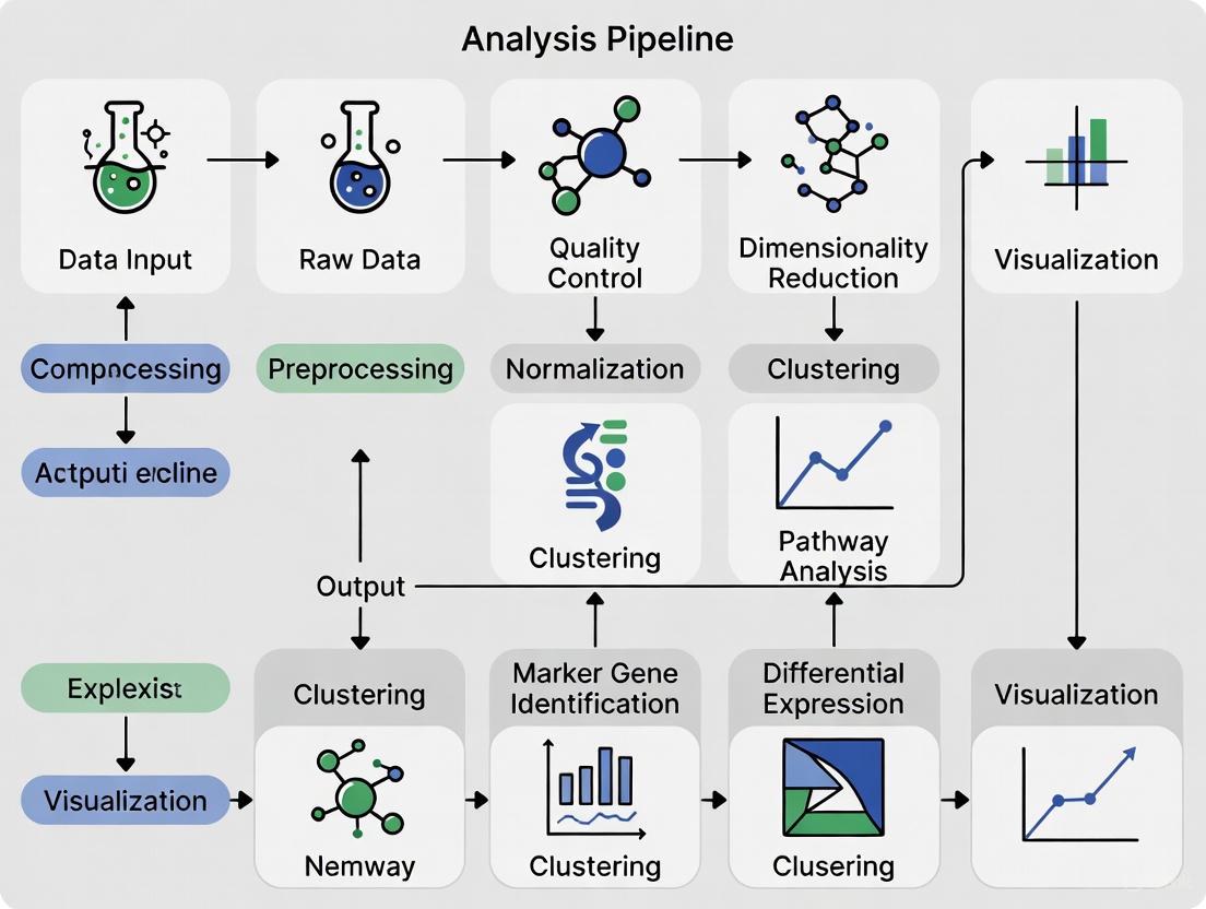
The following DOT script illustrates the computational analysis pipeline:
Advanced Analytical Approaches for Stem Cell Biology
Trajectory Inference and RNA Velocity
Understanding lineage relationships is fundamental to stem cell biology. Trajectory inference methods like Monocle 3 reconstruct developmental paths from scRNA-seq data, ordering cells along pseudotemporal trajectories that represent differentiation processes [16]. The analytical protocol involves:
Trajectory Structure Learning: Monocle 3 uses a graph-based approach to learn the underlying trajectory structure from reduced dimension space.
Branch Analysis: Identification of branch points where cell fate decisions occur, which is critical for understanding lineage specification in stem cell systems.
RNA Velocity Integration: Combining trajectory inference with RNA velocity from Velocyto provides directional information about cellular dynamics, predicting future states of stem cells along the differentiation continuum [16].
Multi-modal Integration and Spatial Context
Recent technological advances enable simultaneous measurement of multiple molecular modalities from the same cells. The computational framework for integrative analysis includes:
Cross-Modality Integration: Seurat's anchoring system enables integration of scRNA-seq with scATAC-seq, protein expression, and spatial data [16].
Spatial Transcriptomics Analysis: Squidpy has emerged as a primary tool for spatial single-cell analysis, offering neighborhood graph construction, ligand-receptor interaction analysis, and spatial clustering [16].
Stem Cell Niche Characterization: Integration of scRNA-seq with spatial data enables mapping of stem cells within their anatomical context, revealing niche interactions that maintain stemness or direct differentiation.
Research Reagent Solutions
Table 3: Essential Research Reagents and Computational Resources
| Resource Type | Specific Tool/Platform | Function | Application in Stem Cell Research |
|---|---|---|---|
| Raw Data Processing | Cell Ranger | Process 10x Genomics data, alignment, quantification | Foundational processing of stem cell scRNA-seq data [16] |
| Programming Environment | R/Python with Seurat/Scanpy | Statistical computing, analysis pipeline implementation | Flexible, customizable analysis of stem cell datasets [16] |
| Reference Databases | CellMarker, PanglaoDB | Cell type annotation references | Identification of stem cell and differentiated cell types [17] |
| Enrichment Analysis | clusterProfiler, GSEA | Functional interpretation of gene sets | Pathway analysis of stem cell signatures [17] |
| Collaborative Platform | CytoAnalyst | Web-based analysis with sharing capabilities | Multi-user stem cell projects, educational use [17] |
The computational landscape for scRNA-seq analysis has matured into a sophisticated ecosystem of interoperable tools and platforms that enable comprehensive investigation of stem cell biology. Foundational platforms such as Scanpy, Seurat, and SingleCellExperiment provide the analytical backbone, while specialized tools address specific challenges such as trajectory inference, RNA velocity, and multi-modal integration. As single-cell technologies continue to evolve toward increasingly multi-modal measurements, computational methods that can integrate across spatial, epigenetic, and transcriptomic data will be essential for unraveling the complex regulatory networks that govern stem cell fate decisions. The field is moving toward tools that are both computationally powerful and biologically interpretable, enabling deeper insights into stem cell biology with direct relevance to regenerative medicine and therapeutic development.
The Analytical Workflow in Action: A Step-by-Step Guide from Raw Data to Biological Insight
Data Pre-processing and Rigorous Quality Control for Stem Cell Datasets
Single-cell RNA sequencing (scRNA-seq) has revolutionized stem cell research by enabling the dissection of cellular heterogeneity and the identification of rare cell populations at unprecedented resolution [11]. Unlike bulk RNA sequencing, which provides population-averaged data, scRNA-seq captures gene expression profiles of individual cells, revealing cell subtypes and dynamic transitions that would otherwise be obscured [19]. However, the minute quantities of starting material and technical artifacts inherent in single-cell protocols introduce specific challenges that necessitate rigorous quality control (QC) and pre-processing pipelines [11]. This application note provides detailed methodologies for data pre-processing and quality control specifically tailored to stem cell scRNA-seq datasets, framed within a comprehensive computational analysis pipeline.
Key Quality Metrics and Thresholds for Stem Cell Data
Quality control begins with the computation and assessment of key metrics that reflect cell viability, sequencing depth, and technical artifacts. The table below summarizes critical QC parameters, their biological interpretations, and recommended filtering thresholds for stem cell datasets.
Table 1: Essential Quality Control Metrics for Stem Cell scRNA-seq Data
| QC Metric | Biological/Technical Interpretation | Recommended Threshold | Stem Cell Specific Considerations |
|---|---|---|---|
| Unique Gene Counts | Sequencing depth & transcriptional activity | Minimum: 200-500; Maximum: 2,500-5,000 [17] | Varies by stem cell type and differentiation state |
| UMI Counts | Capture efficiency & library complexity | Minimum: 500-1,000; Maximum: 10,000-25,000 [17] | High variance may indicate mixed populations |
| Mitochondrial Gene Percentage | Cellular stress & apoptosis | Typically <5-10% [17] | May increase during differentiation; monitor carefully |
| Ribosomal Gene Percentage | Cellular state & translational activity | Variable; often 5-20% | Can indicate specific metabolic states in stem cells |
| Cell Complexity (Genes/UMI) | Technical quality | >0.8 often acceptable | Low values may indicate damaged cells or empty droplets |
For multi-sample stem cell experiments, quality metrics should be computed and visualized independently for each sample to identify batch-specific issues and apply sample-specific filtering thresholds when necessary [17]. Platforms like CytoAnalyst automatically generate interactive violin plots displaying distributions of these metrics across all cells, enabling dynamic threshold adjustment while observing effects on cell populations in real-time [17].
scRNA-seq Protocols: Selection Considerations for Stem Cell Research
The choice of scRNA-seq protocol significantly impacts downstream quality control parameters and analytical approaches. Different methods offer distinct advantages in transcript coverage, cell throughput, and detection sensitivity that must be aligned with stem cell research objectives.
Table 2: Comparison of scRNA-seq Protocols Relevant to Stem Cell Research
| Protocol | Isolation Strategy | Transcript Coverage | UMI | Amplification Method | Stem Cell Research Applications |
|---|---|---|---|---|---|
| Smart-Seq2 [11] | FACS | Full-length | No | PCR | Enhanced sensitivity for low-abundance transcripts; ideal for detecting rare regulatory factors in stem cells |
| Drop-Seq [11] | Droplet-based | 3′-end | Yes | PCR | High-throughput profiling of heterogeneous stem cell populations; cost-effective for large-scale differentiation studies |
| inDrop [11] | Droplet-based | 3′-end | Yes | IVT | Efficient barcode capture; suitable for time-course experiments tracking differentiation trajectories |
| Seq-well [11] | Droplet-based | 3′-only | Yes | PCR | Portable platform for limited stem cell samples; minimal equipment requirements |
| Fluidigm C1 [11] | Microfluidics | Full-length | No | PCR | Precise cell handling for precious stem cell samples; enables integrated genomic analyses |
| SPLiT-Seq [11] | Combinatorial indexing | 3′-only | Yes | PCR | Fixed stem cell samples; eliminates dissociation bias; highly scalable for developmental atlases |
Full-length transcript protocols (Smart-Seq2, Fluidigm C1) offer advantages for isoform usage analysis and detection of allelic expression patterns crucial for understanding regulatory mechanisms in stem cells [11]. Droplet-based methods (Drop-Seq, inDrop) enable higher throughput at lower cost per cell, making them particularly valuable for capturing rare stem cell subtypes and comprehensive differentiation landscapes [11].
Experimental Workflow and Computational Pipeline
The following diagram illustrates the complete scRNA-seq data pre-processing and quality control workflow for stem cell datasets, from sample preparation to analysis-ready data:
Figure 1: scRNA-seq Data Pre-processing and QC Workflow for Stem Cell Research
Research Reagent Solutions for Stem Cell scRNA-seq
The following table details essential research reagents and computational tools critical for implementing robust stem cell scRNA-seq quality control pipelines:
Table 3: Essential Research Reagent Solutions for Stem Cell scRNA-seq QC
| Category | Product/Platform | Specific Function | Application Notes |
|---|---|---|---|
| Wet Lab Protocols | Smart-Seq2 [11] | Full-length transcript amplification | Maximizes detection of low-abundance transcripts; ideal for stem cell regulatory networks |
| Drop-Seq [11] | High-throughput single-cell encapsulation | Enables analysis of thousands of stem cells; identifies rare subpopulations | |
| Computational Tools | CytoAnalyst [17] | Web-based QC and analysis platform | Interactive quality metric visualization; real-time filtering; collaborative analysis |
| LIANA [20] | Ligand-receptor analysis framework | Evaluates cell-cell communication in stem cell niches post-QC | |
| Reference Databases | OmniPath [20] | Cell-cell communication interactions | Contextualizes stem cell signaling within microenvironment |
| CellChatDB [20] | Ligand-receptor interaction repository | Specialized for signaling pathway analysis in development | |
| Quality Control Metrics | Unique Molecular Identifiers (UMIs) [11] | Correction for amplification bias | Essential for accurate transcript quantification in stem cells |
| Mitochondrial gene sets [17] | Cell viability assessment | Critical for detecting stressed cells in stem cell preparations |
Signaling Pathways and Cell-Cell Communication Analysis
Following quality control, analysis of cell-cell communication provides critical insights into stem cell niche interactions and signaling pathways governing self-renewal and differentiation decisions. The following diagram illustrates key signaling pathways identifiable through scRNA-seq data after rigorous QC:
Figure 2: Stem Cell Signaling Pathways Analyzable via scRNA-seq Data
Resources for cell-cell communication inference exhibit varying coverage of key developmental pathways. For instance, the Notch and Wnt pathways—critical for stem cell fate decisions—show significant representation across most resources, though some resources demonstrate underrepresentation of specific pathways like the T-cell receptor pathway, which may be relevant for immune-stem cell interactions [20]. Tools such as LIANA provide a unified framework for accessing multiple resources and methods, enabling comprehensive analysis of stem cell communication landscapes [20].
Implementation Considerations for Stem Cell Research
Successful implementation of scRNA-seq quality control pipelines for stem cell research requires additional considerations specific to stem cell biology. Stem cells often exhibit unique metabolic profiles that impact standard QC thresholds, particularly regarding mitochondrial content. During differentiation, temporary increases in mitochondrial gene percentage may reflect metabolic restructuring rather than cellular stress, necessitating adjusted thresholds or secondary validation [17].
For stem cell applications investigating rare populations or fine differentiation transitions, preprocessing should prioritize sensitivity maintenance. This may involve conservative filtering approaches that prioritize false negatives over false positives, particularly when working with precious stem cell samples. Integration of multiple normalization approaches (e.g., log-normalization and SCTransform) through platforms like CytoAnalyst enables parallel processing and comparison to determine optimal strategies for specific stem cell questions [17].
Batch effect correction requires particular attention in stem cell studies involving multiple differentiation experiments or time courses. Methods such as Harmony, RPCA, or CCA should be systematically evaluated to preserve biologically meaningful variation while removing technical artifacts [17]. The ability to maintain and compare multiple analysis instances facilitates this optimization process.
Rigorous quality control and standardized pre-processing pipelines form the essential foundation for reliable stem cell scRNA-seq research. By implementing the detailed protocols and metrics outlined in this application note, researchers can effectively address technical challenges while maximizing biological insights into stem cell heterogeneity, differentiation trajectories, and niche interactions. The integrated approach combining wet-lab protocols, computational QC tools, and signaling analysis frameworks enables robust interrogation of stem cell systems at single-cell resolution, supporting advances in developmental biology, regenerative medicine, and therapeutic development.
Data Normalization, Integration, and Batch Effect Correction in Multi-Sample Studies
In the context of stem cell scRNA-seq research, multi-sample studies are essential for robustly identifying novel stem cell subpopulations, understanding differentiation dynamics, and mapping developmental trajectories. The computational analysis of such datasets presents significant challenges in distinguishing genuine biological signals, such as transient progenitor states during stem cell differentiation, from technical artifacts introduced during sample processing. Technical variability or "batch effects" can arise from differences in sample preparation personnel, reagent lots, sequencing platforms, or processing dates, which can systematically mask the biological heterogeneity of interest in stem cell populations [21] [22]. Effective data normalization, integration, and batch effect correction therefore form a critical foundation for any computational pipeline aimed at extracting biologically meaningful insights from multi-sample stem cell studies. These preprocessing steps ensure that observed differences in gene expression truly reflect stem cell biology rather than technical confounders, enabling more accurate identification of stem cell states, lineage commitment markers, and molecular signatures of cellular potency.
Data Normalization: Foundations and Methods
The Necessity of Normalization in scRNA-seq Data
Normalization is a critical first step in scRNA-seq analysis that enables meaningful comparison of gene expression levels within and between individual cells. The raw count data generated from sequencing platforms are not directly comparable due to substantial technical variability, particularly in sequencing depth (library size), where orders-of-magnitude differences are commonly observed between cells [23]. Without appropriate normalization, these technical differences can become the dominant source of variation in the data, completely obscuring the biological signals of interest, such as the subtle transcriptional changes that occur during stem cell differentiation.
Single-cell RNA-sequencing data possess distinct characteristics that complicate their analysis, including an unusually high abundance of zero values (dropouts), increased cell-to-cell variability, and complex expression distributions [24]. This high intercellular variability stems from both biological factors (e.g., stochastic gene expression, cell cycle effects) and technical factors (e.g., capture efficiency, amplification bias). Effective normalization must account for these sources of variation while preserving genuine biological heterogeneity, which is particularly important in stem cell research where rare transitional states may be critical for understanding differentiation pathways.
Normalization Methodologies
Table 1: Common scRNA-seq Normalization Methods
| Method | Underlying Principle | Advantages | Limitations | Stem Cell Research Applications |
|---|---|---|---|---|
| CPM | Converts raw counts to counts per million by scaling by total counts | Simple, intuitive calculation | Sensitive to highly expressed genes; assumes total RNA content is constant | Initial data exploration; not recommended for complex multi-sample studies |
| SCTransform | Regularized negative binomial regression on UMIs with library size as covariate | Effectively stabilizes variance; eliminates influence of sequencing depth on PCA | Designed for UMI data; may oversmooth in extremely sparse datasets | Recommended for complex stem cell atlases with multiple samples and conditions |
| Scran | Pooling-based deconvolution approach using linear combinations of cell pools | Robust to zero inflation; handles varying library sizes effectively | Computational intensity increases with sample size | Ideal for heterogeneous stem cell populations with varying RNA content |
| RLE (SF) | Median ratio method using geometric means across cells | Robust to differential expression patterns | Requires sufficient non-zero expression across cells | Suitable for well-sequenced stem cell cultures with lower dropout rates |
| TMM | Weighted trimmed mean of M-values relative to reference sample | Adjusts for RNA composition effects | Assumes most genes are not differentially expressed | Appropriate for controlled differentiation time-course experiments |
| Upper Quartile | Scales counts using upper quantile of expression distribution | Less sensitive to outliers than total sum scaling | Problematic with low-depth data with many zeros | Limited utility for sparse stem cell datasets |
In stem cell research, the choice of normalization method can significantly impact downstream interpretations. For example, when studying heterogeneous populations containing both quiescent and activated stem cells, methods like scran that explicitly account for varying RNA content are preferable [23]. Similarly, when analyzing large-scale stem cell atlases encompassing multiple cell lines and differentiation timepoints, SCTransform has demonstrated superior performance in removing the relationship between technical covariates and biological variation, thereby enhancing the detection of subtle transcriptional states [23].
Batch Effect Correction and Data Integration
Understanding Batch Effects in Multi-Sample Studies
Batch effects represent systematic technical differences between datasets generated under different conditions, at different times, or by different personnel. In stem cell research, these effects are particularly problematic as they can mimic or obscure genuine biological signals, such as differences between stem cell lines, differentiation stages, or experimental conditions. Large scRNA-seq projects inevitably require data generation across multiple batches due to logistical constraints, making batch effect correction an essential step in the analytical pipeline [21].
The challenges of batch effect correction are particularly pronounced in stem cell biology due to the potential for both technical and biological differences between batches. For instance, if different stem cell lines are processed in different batches, it becomes difficult to distinguish expression differences attributable to genuine biological variation from those arising from technical artifacts. Computational removal of batch-to-batch variation enables researchers to combine data across multiple batches for consolidated analysis, thereby increasing statistical power and enabling more comprehensive characterization of stem cell heterogeneity [21].
Integration Strategies for Multi-Sample Data
Table 2: Batch Effect Correction Methods for scRNA-seq Data
| Method | Algorithm Type | Key Features | Data Requirements | Performance Considerations |
|---|---|---|---|---|
| FastMNN | Nearest-neighbor based | Fast, memory-efficient; preserves biological heterogeneity | Requires selection of highly variable genes | High scalability; suitable for large stem cell atlases |
| Harmony | Iterative clustering and integration | Uses PCA for dimension reduction; iterative correction | Works on principal components | Effective for datasets with complex batch structure |
| Seurat (CCA) | Canonical correlation analysis | Identifies shared correlation structures across datasets | Requires comparable cell types across batches | Conservative approach; may retain some batch effects |
| Scanorama | Panorama stitching via mutual nearest neighbors | Handers multiple batches simultaneously | Automatic feature selection | Efficient for integrating multiple timepoints |
| ComBat | Linear model with empirical Bayes | Adjusts for known batches; can include biological covariates | Assumes balanced design across batches | Can be too aggressive if biological differences exist |
| rescaleBatches() | Linear regression | Removes batch effect by scaling batch means; preserves sparsity | Assumes similar population composition | Rapid processing; maintains matrix sparsity |
Several specialized tools have been developed specifically for batch correction of single-cell data that do not require a priori knowledge about cell population composition [21]. This feature is particularly valuable for exploratory analyses of stem cell datasets where the complete spectrum of cellular states may not be fully known in advance. The quickCorrect() function from the batchelor package, for instance, provides a streamlined workflow that performs data preparation, feature selection, and mutual nearest neighbors (MNN) correction in a unified framework [21].
Experimental Protocols and Workflows
Comprehensive Data Preprocessing Protocol
A robust preprocessing pipeline is essential for preparing high-quality stem cell scRNA-seq data for normalization and integration. The following protocol outlines key steps:
Step 1: Quality Control and Filtering
- Calculate quality metrics: Count depth, number of detected genes per cell, and mitochondrial read fraction [25]
- Identify and remove low-quality cells using multivariate thresholding
- Filter out droplets with unusually high UMI counts (potential multiplets) or high mitochondrial content (dying cells) [22]
- Expected outcomes: For healthy stem cell populations, mitochondrial percentage typically below 10-20%; minimum gene detection threshold varies by platform
Step 2: Normalization Implementation
- Select appropriate normalization method based on data characteristics (refer to Table 1)
- For scran: Apply quick clustering and compute size factors using
computeSumFactors() - For SCTransform: Run
SCTransform()with default parameters for UMI data - Validate normalization effectiveness by examining the relationship between technical covariates and principal components
Step 3: Feature Selection
- Identify highly variable genes (HVGs) using variance-stabilizing transformation
- Select 2,000-5,000 most variable genes for downstream analysis
- For multi-sample studies: Use
combineVar()to average variance components across batches [21]
Step 4: Batch Correction
- Select integration method based on study design (refer to Table 2)
- For FastMNN: Run
fastMNN()on selected HVGs - For Harmony: Apply
RunHarmony()on PCA embeddings - Validate integration using cluster-specific batch mixing metrics
Step 5: Downstream Analysis
- Perform dimensionality reduction (PCA, UMAP, t-SNE) on integrated data
- Conduct clustering analysis using graph-based or density-based methods
- Identify cluster markers and annotate cell types
- Perform differential expression analysis across conditions
Multi-Sample Integration Protocol
For studies involving multiple stem cell samples, the following specialized protocol ensures effective integration:
Sample Preparation and Preprocessing
- Process each sample individually through QC and basic normalization
- Use
multiBatchNorm()to rescale batches and adjust for systematic differences in coverage [21] - Subset all batches to the common feature space
Feature Selection for Integration
- Perform feature selection using
combineVar()to average variance components across batches - Select a larger number of HVGs (e.g., 5,000) than typical single-dataset analyses
- This ensures retention of markers for sample-specific subpopulations that might be present
Integration Execution
- Choose correction algorithm based on dataset characteristics (see Table 2)
- For
quickCorrect(): Apply to multiple SingleCellExperiment objects with specified HVGs - Assess integration quality by examining mixing of batches in low-dimensional embeddings
Integration Quality Assessment
- Visualize batch distribution across clusters
- Calculate integration metrics (e.g., local inverse Simpson's index)
- Confirm preservation of biological variation while removing technical artifacts
The Scientist's Toolkit: Essential Research Reagents and Computational Tools
Table 3: Essential Computational Tools for scRNA-seq Data Processing
| Tool/Package | Primary Function | Application Context | Key Features | Implementation |
|---|---|---|---|---|
| Scran | Normalization using pooled size factors | Single-cell specific normalization | Robust to zero inflation; deconvolution approach | R/Bioconductor |
| SCTransform | Normalization and variance stabilization | UMI-based datasets | Regularized negative binomial regression; eliminates depth influence | R/Seurat |
| batchelor | Batch correction using MNN | Multi-sample integration | FastMNN implementation; preserves biological heterogeneity | R/Bioconductor |
| Seurat | Comprehensive analysis suite | End-to-end workflow | CCA integration; SCTransform normalization; extensive visualization | R |
| Scanpy | Single-cell analysis in Python | Python-based workflows | BBKNN integration; scalable to very large datasets | Python |
| Harmony | Batch integration | Complex batch structures | Iterative clustering and correction; works on embeddings | R/Python |
| Cell Ranger | Primary data processing | 10x Genomics data | Alignment, barcode processing, count matrix generation | Command line |
Applications in Stem Cell Research
The normalization and integration methodologies described in this article enable several critical applications in stem cell biology. In developmental patterning studies, effective batch correction allows researchers to integrate scRNA-seq data from multiple embryonic timepoints, revealing continuous differentiation trajectories and identifying transient progenitor populations that would be impossible to detect in individual samples [11]. For disease modeling using induced pluripotent stem cells (iPSCs), these computational approaches enable robust comparison of patient-derived lines and controls, facilitating the identification of disease-relevant transcriptional signatures despite technical variability introduced during cellular reprogramming and differentiation.
In drug discovery applications, multi-sample integration methods allow researchers to combine scRNA-seq data from compound screening experiments conducted at different times or locations. This enables comprehensive assessment of how small molecules or biologics affect stem cell differentiation patterns and transcriptional states, accelerating the identification of compounds that direct stem cells toward therapeutic relevant fates [11]. Furthermore, as single-cell technologies continue to evolve toward multi-omic profiling, the normalization and integration frameworks established for transcriptomic data will provide a foundation for analyzing integrated datasets that simultaneously capture gene expression, chromatin accessibility, and protein abundance in stem cell populations.
Data normalization, integration, and batch effect correction constitute essential components of the computational analysis pipeline for stem cell scRNA-seq research. The methodologies and protocols outlined in this article provide a structured framework for addressing the technical challenges inherent in multi-sample studies, enabling researchers to focus on the biological questions of interest. As single-cell technologies continue to advance, producing increasingly large and complex datasets, the development of more sophisticated normalization and integration approaches will be crucial for unlocking the full potential of stem cell transcriptomics. By implementing these best practices, researchers can ensure that their findings reflect genuine stem cell biology rather than technical artifacts, accelerating progress in both basic stem cell biology and translational applications.
Dimensionality Reduction and Clustering to Uncover Distinct Stem Cell Subpopulations
A primary challenge in stem cell biology is the inherent heterogeneity within seemingly uniform cell populations [26]. Single-cell RNA sequencing (scRNA-seq) has emerged as a pivotal technology for deconvoluting this complexity, enabling researchers to measure the expression of thousands of genes across thousands of individual cells [27]. However, the high-dimensional, sparse, and noisy nature of scRNA-seq data necessitates robust computational methods for distillation and interpretation [27] [28]. Dimensionality reduction and clustering are two critical, interdependent steps in the downstream analysis pipeline that allow scientists to project data into an intelligible low-dimensional space and identify groups of cells with similar transcriptomic profiles, potentially representing distinct stem cell states, lineages, or functional subpopulations [27] [29]. Within the broader context of developing a computational pipeline for stem cell research, this protocol details the application of these methods to uncover biologically meaningful subpopulations, a capability with profound implications for understanding development, regeneration, and drug discovery.
Computational Methodology
Dimensionality reduction methods transform high-dimensional gene expression data into a lower-dimensional representation, preserving key patterns of cellular heterogeneity. These methods can be broadly categorized as follows:
- Linear Methods: These include classic techniques like Principal Component Analysis (PCA), which identifies the linear combinations of genes (principal components) that account for the maximum variance in the data [27] [30]. PCA is widely used as an initial denoising and data compression step.
- Non-Linear Methods: Designed to capture more complex, non-linear relationships in the data. t-Distributed Stochastic Neighbor Embedding (t-SNE) excels at revealing local structure and is known for producing visually distinct clusters [27] [30]. Uniform Manifold Approximation and Projection (UMAP) often preserves more of the global data structure than t-SNE and offers superior run-time performance, making it a current standard for visualization [27] [29].
- Model-Based and Neural Network Methods: These approaches explicitly model characteristics of scRNA-seq data. Zero-Inflated Factor Analysis (ZIFA) incorporates a model for dropout events [27]. More recently, deep learning models like Variational Autoencoders (VAEs) and the Boosting Autoencoder (BAE) offer powerful, flexible frameworks for non-linear dimension reduction that can incorporate structural assumptions, such as enforcing sparsity to identify small, explanatory gene sets [27] [31].
Table 1: Comparison of Common Dimensionality Reduction Methods for scRNA-seq Data
| Method | Category | Key Features | Best Use-Case | Considerations |
|---|---|---|---|---|
| PCA [27] [30] | Linear | Fast, simple, computationally efficient. | Initial data compression and denoising. | May miss non-linear biological relationships. |
| t-SNE [27] | Non-linear | Excellent at revealing local structure and fine-grained clustering. | Visualizing distinct cell populations. | Computationally expensive; preserves local over global structure. |
| UMAP [27] [29] | Non-linear | Preserves more global structure than t-SNE; faster. | General-purpose visualization for large datasets. | Parameters can influence results; requires tuning. |
| ZIFA [27] | Model-based | Accounts for "dropout" events (zero inflation). | Data with high levels of technical noise. | Higher computational complexity than PCA. |
| BAE [31] | Neural Network | Identifies small gene sets for each dimension; incorporates constraints. | Finding sparse marker genes for specific subpopulations. | More complex implementation; requires customization. |
Clustering Strategies for Subpopulation Identification
Following dimensionality reduction, clustering algorithms group cells based on the similarity of their low-dimensional representations. The choice of algorithm can significantly impact the subpopulations discovered.
- K-means: A partition-based method that assigns cells to a user-specified number (k) of clusters by iteratively identifying cluster centers [29] [30]. It is useful for an initial assessment but requires prior knowledge of the expected number of clusters.
- Graph-based Clustering: This method partitions data into clusters based on the data's inherent structure (e.g., community detection in a cell-cell graph) rather than a predefined number [30]. It is highly effective for identifying complex population structures and is a default in many modern toolkits.
- Joint Dimension Reduction and Clustering: Emerging methods like DR-SC and DcjComm unify these two steps within a single statistical framework [28] [29]. This ensures that the low-dimensional features extracted are directly relevant to the cluster labels inferred, often leading to improved performance and more biologically meaningful results.
The following diagram illustrates the standard sequential workflow compared to an integrated joint analysis approach.
Detailed Protocol for Subpopulation Analysis
This section provides a step-by-step protocol for analyzing scRNA-seq data from stem cells to identify distinct subpopulations, utilizing popular computational frameworks.
Data Preprocessing and Quality Control
- Load Data: Begin by loading the filtered cell-feature matrix (e.g., the output from the Cell Ranger pipeline) into your analysis environment of choice, such as R/Seurat or Python/Scanpy [16] [30].
- Quality Control (QC): Filter the data to remove low-quality cells and genes.
- Remove cells with an abnormally high number of detected genes (potential doublets) or a high percentage of mitochondrial reads (indicative of apoptotic or stressed cells).
- Filter out genes that are detected in only a very small number of cells.
- Normalization and Scaling: Normalize the gene expression counts for each cell by the total expression, multiply by a scale factor (e.g., 10,000), and log-transform the result. Scale the data to give equal weight to highly and lowly variable genes in downstream steps.
Dimensionality Reduction and Clustering
- Feature Selection: Identify a subset of highly variable genes (HVGs) that drive heterogeneity across the cell population. This focuses the downstream analysis on the most biologically relevant features.
- Linear Dimension Reduction: Perform PCA on the scaled data of HVGs. Use the top principal components (PCs) for subsequent analysis, as they capture the majority of the meaningful variance.
- Neighborhood Graph Construction: Based on the PCA reduction, construct a graph where each cell is a node and edges are drawn between cells with similar expression profiles (e.g., using k-nearest neighbors).
- Non-Linear Visualization: Generate UMAP or t-SNE plots using the neighborhood graph to visualize the data in 2D or 3D.
- Clustering: Apply a graph-based clustering algorithm (e.g., Louvain, Leiden) to the neighborhood graph to partition cells into discrete groups. The resolution parameter can be adjusted to control the granularity of the clusters, with lower resolution yielding broader and higher resolution yielding finer clusters.
Biological Interpretation and Validation
- Differential Expression (DE): For each cluster, perform DE analysis to identify genes that are significantly upregulated compared to all other clusters. These serve as potential marker genes for the subpopulation.
- Cell Type Annotation: Manually annotate clusters by comparing the identified marker genes to known canonical markers from the literature (e.g., CD44, CD73, CD90, CD105 for mesenchymal stem cells [26]).
- Validation with Functional Assays: Computational predictions require experimental validation. For instance, subpopulations identified by scRNA-seq can be isolated using Fluorescence-Activated Cell Sorting (FACS) based on surface markers revealed by the analysis, followed by functional assays to confirm distinct properties like proliferative capacity or differentiation potential [26] [32].
Table 2: The Scientist's Toolkit: Essential Reagents and Tools for scRNA-seq Subpopulation Analysis
| Item | Function/Description | Example/Reference |
|---|---|---|
| 10x Genomics Chromium | A widely used platform for generating single-cell libraries for sequencing. | Cell Ranger [16] [30] |
| Seurat / Scanpy | Comprehensive software toolkits for the analysis of single-cell genomics data. | Seurat (R), Scanpy (Python) [16] |
| Reference Transcriptome | A pre-assembled set of genomic sequences for aligning sequencing reads to identify transcripts. | ENSEMBL, GENCODE [30] |
| Fluorescently-Labeled Antibodies | Reagents for isolating specific cell subpopulations via FACS for downstream validation. | Anti-CD44, Anti-CD90 [26] [32] |
| Cell Culture Reagents | Media and supplements for the maintenance and differentiation of stem cell cultures. | αMEM with human serum [26] |
Advanced Applications and Integrated Analysis
The basic workflow can be extended to address more complex biological questions, particularly with the integration of additional data modalities.
Identifying Small and Rare Subpopulations
Advanced methods like the Boosting Autoencoder (BAE) are particularly adept at identifying small gene sets that characterize very small cell groups with distinct transcriptomic signatures, which might be lost in a global clustering analysis [31]. By enforcing sparsity, BAE ensures that different latent dimensions are driven by small, non-overlapping sets of genes, which can be directly interpreted as marker genes for specific subpopulations, including rare ones.
Integrating scRNA-seq with Spatial Transcriptomics
The combination of scRNA-seq with spatial transcriptomics technologies allows researchers to not only identify subpopulations but also understand their spatial organization—a critical aspect of stem cell niches. Computational methods like Squidpy and SpaGCN are designed to analyze spatial transcriptomics data, enabling the identification of spatial domains and the analysis of cell-cell communication within a tissue context [16] [29]. The following diagram outlines how these data types can be integrated.
Inferring Cell-Cell Communication
Subpopulation identity is not only defined by intrinsic gene expression but also by extrinsic signaling. Tools like DcjComm and CellChat can infer cell-cell communication (CCC) networks by integrating the expression of ligand-receptor pairs between computationally defined subpopulations [29]. This provides a systems-level view of the signaling microenvironment that maintains stem cell states or drives their fate decisions.
Differential Expression Analysis and Marker Gene Identification
Single-cell RNA sequencing (scRNA-seq) has revolutionized the study of cellular heterogeneity, proving particularly transformative for stem cell biology. This technology enables the dissection of complex populations of hematopoietic stem and progenitor cells (HSPCs), revealing previously inaccessible developmental trajectories and molecular mechanisms governing cell fate decisions [33]. Within this context, differential expression (DE) analysis and marker gene identification form the computational cornerstone for translating raw sequencing data into biologically meaningful insights. These analyses allow researchers to identify distinct transcriptional programs between cell states, pinpoint regulatory networks maintaining stemness, and uncover molecular drivers of differentiation. The application of these methods to stem cell research, however, presents unique challenges, including the need to work with limited cell numbers and to distinguish subtle transcriptional differences in primed progenitor populations [33] [34]. This protocol details a robust pipeline for performing DE analysis and marker gene identification specifically optimized for stem cell scRNA-seq datasets, integrating best practices from current literature to ensure sensitive and biologically-relevant results.
Experimental and Computational Protocols
Wet-Lab Protocol: Stem Cell Preparation and Sequencing
Cell Isolation and Sorting (Adapted from Human HSPC Workflow) [33]
- Sample Source: Obtain human umbilical cord blood (hUCB) with appropriate ethical approval and donor consent.
- Mononuclear Cell Isolation: Dilute hUCB with phosphate-buffered saline (PBS) and carefully layer over Ficoll-Paque density gradient medium. Centrifuge for 30 minutes at 400× g at 4°C. Collect the mononuclear cell (MNC) layer, wash, and resuspend.
- Fluorescent-Activated Cell Sorting (FACS): Stain the MNCs with a cocktail of antibodies. A typical panel for HSPC enrichment includes:
- Positive Selection: Antibodies against CD34 (PE-conjugated) and/or CD133 (APC-conjugated), and CD45 (PE-Cy7-conjugated).
- Negative Selection (Lineage Depletion): A cocktail of FITC-conjugated antibodies against lineage-specific markers (e.g., CD235a, CD2, CD3, CD14, CD16, CD19, CD24, CD56, CD66b).
- Gating Strategy: On a flow cytometer (e.g., MoFlo Astrios EQ), first gate small, lymphocyte-like events (2–15 μm). From this population (P1), select Lin¯ negative events. Finally, sort the CD34+Lin¯CD45+ and/or CD133+Lin¯CD45+ populations directly into a suitable collection medium [33].
Table 1: Key Research Reagent Solutions for Stem Cell scRNA-seq
| Item | Function | Example & Specification |
|---|---|---|
| Ficoll-Paque | Density gradient medium for mononuclear cell isolation | GE Healthcare Ficoll-Paque PLUS [33] |
| Lineage Cocktail Antibodies | Negative selection to deplete differentiated cells | FITC-conjugated anti-CD235a, CD2, CD3, etc. [33] |
| CD34 & CD133 Antibodies | Positive selection for hematopoietic stem/progenitor cells | PE-anti-CD34, APC-anti-CD133 [33] |
| Cell Sorter | Isolation of highly pure stem cell populations | Beckman Coulter MoFlo Astrios EQ [33] |
| Single-Cell Library Kit | Generation of barcoded scRNA-seq libraries | 10X Genomics Chromium Next GEM Single Cell 3' Kit v3.1 [33] |
Single-Cell Library Preparation and Sequencing
- Immediately process sorted cells using a platform such as the 10X Genomics Chromium Controller.
- Use the Chromium Next GEM Single Cell 3' Reagent Kit for library preparation, strictly following the manufacturer's guidelines.
- Pool libraries and sequence on an Illumina platform (e.g., NextSeq 1000/2000) using a P2 flow cell (200 cycles) in paired-end mode, targeting a minimum of 25,000 reads per cell [33].
Computational Protocol: Data Processing and DE Analysis
Primary Data Processing [35]
- Demultiplexing and Alignment: Process raw BCL files using
cellranger mkfastq(Cell Ranger v7.2.0) to generate FASTQ files. Then, usecellranger countto align reads to the appropriate reference genome (e.g., GRCh38 for human) and generate feature-barcode matrices. - Quality Control (QC): Perform rigorous QC filtering on the cell barcode matrix. The following thresholds are recommended starting points, which should be adjusted based on data inspection:
Differential Expression Analysis Workflow in Seurat
The following steps are implemented in R using the Seurat package (version 5.0.1) [36] [33].
- Data Normalization: Normalize the gene expression data using the
SCTransformfunction, which also performs variance stabilization. - Integration & Clustering: Perform linear dimensionality reduction (PCA) on the normalized data. Identify neighbors and cluster cells using a graph-based algorithm (e.g., Louvain, Leiden) at a chosen resolution. Generate UMAP plots for visualization.
- Marker Gene Identification: Use the
FindAllMarkersfunction to identify genes that are differentially expressed in each cluster compared to all other clusters. Key parameters include:only.pos = TRUE: To identify only genes that are positively enriched in the cluster of interest.logfc.threshold = 0.25: A minimum log-fold change threshold.min.pct = 0.1: A gene must be detected in a minimum fraction of cells in either of the two populations being compared.
- Differential Expression Between Conditions: To compare a specific cell type (e.g., Cluster 1) between two experimental conditions (e.g., treated vs. control), subset the object to include only the cells from that cluster. Then, use the
FindMarkersfunction on the subset object, specifying thegroup.byvariable as the condition metadata.
Diagram 1: scRNA-seq DE analysis workflow.
Quantitative Benchmarks and Data Interpretation
Statistical Considerations for Robust DE Analysis
The sensitivity of DE analysis in scRNA-seq is heavily dependent on the number of cells in the cluster or group being tested. Findings from a systematic study provide a critical quantitative reference for experimental design and interpretation [34]:
Table 2: Cell Number Requirements for Robust DEG Identification [34]
| Target Differential Expression Profile | Minimum Recommended Cells per Cluster | Sensitivity Expectation | ||
|---|---|---|---|---|
| Genes with extreme statistical significance (e.g., unadjusted p < 2.8 × 10⁻²⁴) or high transcript abundance (> 221 TPM) | 50 - 100 cells | > 50% of DEGs identified by bulk RNA-seq | ||
| Genes with modest differences (e.g., as found in perturbed states; adjusted p < 0.05, | log₂FC | 0.5-2) | 2,000 cells | ~60% of DEGs identified by bulk RNA-seq |
| Majority of DEGs identified in a bulk RNA-seq analysis of purified populations | 2,000+ cells | Identify the majority of bulk-identified DEGs |
These benchmarks highlight that studies aiming to detect subtle transcriptional changes within a stem cell population must be designed to capture a sufficient number of cells. Clusters with fewer than 100 cells should be interpreted with extreme caution, as a lack of significant DEGs may reflect low statistical power rather than biological reality [34].
Integration with Stemness Prediction
For stem cell research, DE analysis can be powerfully integrated with computational stemness prediction tools. A common approach is to use a tool like CytoTRACE to predict the stemness or differentiation state of each cell based on its transcriptome [36]. Following this:
- Cells can be grouped based on CytoTRACE-predicted stemness scores (e.g., high-stemness vs. low-stemness clusters).
FindMarkersis then used to perform DE analysis between these groups.- The resulting gene list constitutes a tumor stem cell marker signature (TSCMS) in cancer studies, or a stemness signature in developmental contexts. This signature can be used for prognostic model construction and functional enrichment analysis to understand the biological processes associated with the stem-like state [36].
Diagram 2: Stemness analysis integration.
The Scientist's Toolkit
Table 3: Essential Computational Tools for DE Analysis
| Tool / Resource | Category | Primary Function | Application Note |
|---|---|---|---|
| Cell Ranger [35] | Pipeline | Primary analysis of 10X Genomics data (alignment, barcode counting). | Foundational step; generates the input matrix for all downstream analysis. |
| Seurat [36] [33] | R Toolkit | Comprehensive scRNA-seq analysis, including normalization, clustering, and DE analysis. | The FindMarkers function (using Wilcoxon Rank Sum test) is the workhorse for DE. |
| CytoTRACE [36] | Stemness Prediction | Predicts cellular stemness/differentiation status from scRNA-seq data. | Crucial for defining stem-like populations for comparison in stem cell studies. |
| CytoAnalyst [17] | Web Platform | User-friendly platform for integrated scRNA-seq analysis, from QC to DE and annotation. | Ideal for researchers without extensive coding experience; facilitates reproducibility. |
| scGraphformer [37] | Cell Classification | Transformer-based graph neural network for enhanced cell type identification. | Can improve initial cell typing, leading to more accurate group definitions for DE. |
| SoupX / CellBender [35] | Ambient RNA Removal | Computational removal of background RNA contamination. | Improves data quality, especially for detecting lowly-expressed marker genes. |
Single-cell RNA sequencing (scRNA-seq) has revolutionized our understanding of stem cell biology by enabling the transcriptomic analysis of individual cells within complex populations. Unlike bulk RNA sequencing, which averages gene expression across thousands of cells, scRNA-seq reveals cellular heterogeneity, identifies rare subpopulations, and uncovers dynamic transitions that would otherwise be obscured [19]. This technological advancement is particularly valuable for studying stem cell dynamics, where cellular heterogeneity and fate decisions drive development, tissue regeneration, and disease progression.
In stem cell research, three advanced analytical applications have proven indispensable: cell annotation, trajectory inference, and RNA velocity analysis. Cell annotation enables the precise identification of stem cell states and subtypes within heterogeneous cultures. Trajectory inference reconstructs developmental pathways, ordering cells along pseudotemporal trajectories to model differentiation processes. RNA velocity goes beyond static snapshots by predicting future transcriptional states from unspliced and spliced mRNA ratios, providing direct insights into the dynamics of cell fate decisions [38]. Together, these methods form a comprehensive computational pipeline for unraveling the complexity of stem cell systems, from characterizing cellular identities to modeling temporal dynamics and directional fate choices.
Cell Annotation: Defining Cellular Identities
Principles and Methodologies
Cell annotation is the foundational process of labeling individual cells with biological identities—such as cell types, states, or lineages—based on their transcriptomic profiles. In stem cell research, accurate annotation is crucial for distinguishing between pluripotent states, progenitor cells, and differentiated progeny within heterogeneous populations. The process typically begins with quality control, normalization, and clustering of scRNA-seq data to group transcriptionally similar cells. Annotation is then performed by comparing these clusters to known reference datasets using marker genes, statistical classifiers, or correlation-based approaches [11].
Manual annotation based on canonical marker genes remains widely used but requires expert knowledge and may miss novel cell states. Automated approaches have emerged to address this limitation, leveraging curated reference atlases and machine learning classifiers to assign cell identities with minimal human intervention. The accuracy of cell annotation profoundly impacts all downstream analyses, including trajectory inference and differential expression testing, making robust methodology essential for reliable biological interpretation.
Experimental Protocol for Cell Annotation
Sample Preparation and Sequencing
- Isolate viable single cells from stem cell cultures using fluorescence-activated cell sorting (FACS) or microfluidic partitioning [11] [39].
- Prepare scRNA-seq libraries using 3' or 5' end-counting protocols (e.g., 10x Genomics Chromium platform) for high-throughput analysis or full-length protocols (e.g., Smart-Seq2) for enhanced detection of low-abundance transcripts [11].
- Sequence libraries to a minimum depth of 50,000 reads per cell to ensure adequate transcript detection.
Computational Analysis Workflow
- Quality Control: Filter out low-quality cells with high mitochondrial RNA content (>20%), low unique gene counts (<200 genes), or small numbers of detected molecules.
- Normalization: Apply scRNA-seq-specific normalization methods (e.g., SCTransform) to account for technical variation in sequencing depth.
- Feature Selection: Identify highly variable genes (2,000-3,000 genes) that drive biological heterogeneity.
- Dimensionality Reduction: Perform principal component analysis (PCA) followed by nonlinear methods (UMAP, t-SNE) for visualization.
- Clustering: Apply graph-based clustering algorithms (e.g., Louvain, Leiden) to identify transcriptionally distinct cell groups.
- Annotation: Label clusters using known marker genes, reference dataset integration (e.g., with Seurat's label transfer), or automated classifiers (e.g., SingleR).
Validation
- Validate annotations using independent methods such as immunofluorescence or flow cytometry for key marker proteins.
- Perform differential expression analysis between clusters to confirm distinct transcriptional identities.
Research Reagent Solutions for Cell Annotation
Table 1: Essential Research Reagents for scRNA-seq in Stem Cell Research
| Reagent/Category | Specific Examples | Function in Experimental Workflow |
|---|---|---|
| Cell Isolation | FACS systems, Microfluidic chips (10x Genomics) | Physical separation of single cells for sequencing [11] [39] |
| Library Preparation | 10x Chromium reagents, Smart-Seq2 kits | Barcoding, reverse transcription, and cDNA amplification [11] |
| Sequencing | Illumina sequencing kits | High-throughput reading of cDNA libraries [39] |
| Reference Datasets | Human Cell Atlas, Mouse Cell Atlas | Curated cell type signatures for annotation |
| Analysis Pipelines | Cell Ranger, Seurat, Scanpy | Processing, clustering, and annotation of scRNA-seq data [39] |
Trajectory Inference: Mapping Developmental Pathways
Theoretical Framework
Trajectory inference (TI) methods computationally reconstruct developmental processes by ordering individual cells along pseudotemporal trajectories based on transcriptional similarity [40]. In stem cell biology, TI enables researchers to model differentiation pathways, identify branching points where lineage decisions occur, and discover intermediate cell states that may be transient and rare in vivo. Unlike physical time, pseudotime represents a cell's relative progression through a biological process, with the trajectory origin typically set to the earliest or undifferentiated state [41].
TI methods generally fall into three categories: graph-based approaches (e.g., Monocle, Slingshot) that construct cell-to-cell networks; tree-based methods that build minimum spanning trees; and RNA velocity-assisted approaches that incorporate directional information from spliced/unspliced mRNA ratios [40]. The selection of an appropriate TI method depends on the expected trajectory topology—whether linear (simple differentiation), bifurcating (two lineage choices), or multifurcating (multiple fate decisions)—which is often informed by prior biological knowledge.
Protocol for Trajectory Inference
Preprocessing Requirements
- Start with a properly annotated scRNA-seq dataset containing relevant cell states.
- Subset the data to include only cells participating in the dynamic process of interest.
- Re-perform dimensionality reduction (PCA, UMAP) on the subsetted data to better capture transitions.
Trajectory Inference with tradeSeq
- Input Preparation: Obtain pseudotime values and cell lineage assignments using trajectory inference methods like Slingshot [42].
- Model Fitting: Apply tradeSeq to fit negative binomial generalized additive models (NB-GAMs) that model gene expression as a smooth function of pseudotime across lineages [42].
- Differential Expression Testing:
- Test for association between gene expression and pseudotime within lineages.
- Compare expression patterns between lineages to identify branching-dependent genes.
- Detect genes with different expression patterns between earlier and later trajectory segments.
- Interpretation: Identify genes significantly associated with specific lineage decisions or developmental stages for functional validation.
Ensemble Methods for Robust Inference
- For enhanced robustness, apply the scTEP framework which utilizes multiple clustering results to infer ensemble pseudotime, reducing errors from individual clustering runs [40].
- Use scTEP to fine-tune trajectory graphs by sorting vertices according to average pseudotime, improving trajectory accuracy.
Validation Approaches
- Validate trajectory topology using known marker genes that exhibit sequential expression patterns.
- Confirm pseudotemporal ordering with external data sources (e.g., time-course experiments) when available.
- Use RNA velocity as an orthogonal method to verify inferred directionality.
Trajectory Inference Workflow
Figure 1: Computational workflow for trajectory inference analysis incorporating tradeSeq for differential expression testing.
RNA Velocity: Predicting Cellular Futures
Conceptual Foundations
RNA velocity represents a breakthrough in modeling cellular dynamics from standard scRNA-seq data by quantifying the time derivative of spliced mRNA abundance [38]. The approach leverages the intrinsic kinetics of RNA processing, distinguishing between nascent unspliced pre-mRNA and mature spliced mRNA to predict immediate future transcriptional states of individual cells. Conceptually, an excess of unspliced relative to spliced mRNA indicates upcoming gene upregulation, while a deficit suggests future downregulation [43].
The original RNA velocity model assumed constant transcription, splicing, and degradation rates, but newer methods have substantially advanced this framework. Tools like scVelo introduced likelihood-based dynamical modeling that relaxes the steady-state assumption and infers gene-specific timescales [44]. More recently, deep learning approaches such as veloVI (velocity variational inference) employ generative modeling to provide uncertainty quantification and improve consistency across transcriptionally similar cells [44]. These developments have made RNA velocity particularly valuable for studying stem cell systems, where it can predict fate biases in progenitor cells and characterize transition states during differentiation.
Protocol for RNA Velocity Analysis
Data Requirements
- scRNA-seq data must include both spliced and unspliced counts for each gene.
- Use quantification tools (e.g., velocyto, kallisto) that retain unspliced/unspliced information.
- Ensure sufficient sequencing depth to detect unspliced transcripts, which are typically less abundant.
Velocity Estimation with veloVI
- Model Setup: Implement veloVI, a deep generative model that learns a gene-specific dynamical model of RNA metabolism using a variational autoencoder framework [44].
- Training: Optimize model parameters simultaneously using gradient-based procedures. veloVI provides substantial speed-up compared to EM-based methods (5x faster for 20,000 cells) [44].
- Uncertainty Quantification: Utilize veloVI's posterior distribution over velocities to assess confidence in direction estimates at single-cell resolution.
- Visualization: Project velocity vectors into low-dimensional embeddings (UMAP, t-SNE) to visualize predicted cellular trajectories.
Cluster-Level Direction Inference with TIVelo
- As an alternative approach, implement TIVelo which first determines velocity direction at the cluster level before estimating single-cell velocities [43].
- Main Path Selection: Construct a cluster graph and identify terminal states most likely to be root/end clusters.
- Orientation Inference: Calculate orientation scores based on the principle that unspliced RNA changes precede spliced RNA changes along pseudotime.
- Direction Assignment: Assign levels to clusters and construct directed nearest neighborhoods for single-cell velocity estimation.
Integration with Trajectory Inference
- Combine RNA velocity with trajectory inference methods to reinforce pseudotemporal ordering with directional information.
- Use velocity streamplots to validate and refine trajectory topology, particularly at branching points.
- Identify driver genes of fate decisions by comparing velocity patterns across lineages.
RNA Velocity Analysis Workflow
Figure 2: Comparative workflow for RNA velocity analysis using either veloVI's deep generative modeling or TIVelo's cluster-level direction inference.
Integrated Analysis of Stem Cell Dynamics
Multi-Method Integration Strategy
The true power of advanced scRNA-seq analysis emerges from the integration of cell annotation, trajectory inference, and RNA velocity. This integrated approach provides a comprehensive understanding of stem cell systems, where static classifications are enhanced with dynamic and directional information. The sequential application of these methods creates a pipeline that progresses from identifying cell states to modeling their transitions and predicting their fate commitments.
A robust integration strategy begins with careful experimental design to ensure data quality suitable for all analytical approaches. This includes sufficient cell numbers to capture rare transitions, adequate sequencing depth for unspliced mRNA detection, and appropriate time points or conditions to capture dynamic processes. Computational integration then leverages the complementary strengths of each method: cell annotation provides the biological context for trajectory inference, which in turn establishes a framework for interpreting RNA velocity patterns. Consistency between methods strengthens biological conclusions, while discrepancies may indicate technical artifacts or biologically meaningful complexities worth further investigation.
Comparative Analysis of Computational Tools
Table 2: Comparative Analysis of Advanced scRNA-seq Computational Tools
| Tool | Primary Function | Methodology | Key Advantages | Stem Cell Applications |
|---|---|---|---|---|
| tradeSeq [42] | Trajectory-based DE | Negative binomial GAMs | Tests within-lineage and between-lineage expression patterns | Identifying lineage-specifying genes in differentiation |
| veloVI [44] | RNA velocity | Deep generative modeling | Uncertainty quantification, improved consistency | Predicting fate biases in progenitor cells |
| scTEP [40] | Trajectory inference | Ensemble pseudotime | Robust to clustering errors | Accurate lineage reconstruction in complex differentiation |
| TIVelo [43] | RNA velocity | Cluster-level direction inference | Avoids simple ODE assumptions | Capturing complex transcriptional patterns in development |
| Chronocell [41] | Process time inference | Biophysical model | Interpretable parameters with physical meaning | Linking transcriptomic dynamics to biological time |
Applications in Stem Cell Research
Pluripotency and Early Lineage Specification Integrated scRNA-seq analysis has revealed the transcriptional continuum between naive, primed, and formative pluripotent states in embryonic stem cells. Trajectory inference has mapped the transition routes between these states, while RNA velocity has predicted stabilization points and directionality in pluripotency exit. These insights have practical implications for optimizing stem cell culture conditions and directing differentiation toward specific lineages.
Organoid Development and Maturation In organoid systems, cell annotation identifies emergent cell types, trajectory inference reconstructs the developmental hierarchies that recapitulate organogenesis, and RNA velocity predicts patterning centers and morphogenetic signaling. This integrated approach has been instrumental in improving organoid fidelity by identifying missing cell types and maturation barriers.
Disease Modeling and Regenerative Medicine For disease modeling with patient-specific stem cells, these methods can identify pathological cellular states, map aberrant differentiation pathways, and predict disease-associated fate biases. In regenerative medicine applications, they can assess the equivalence between differentiated cells and their in vivo counterparts, and optimize reprogramming protocols by characterizing intermediate states.
The integration of cell annotation, trajectory inference, and RNA velocity represents a powerful framework for advancing stem cell research. These computational approaches transform static snapshots of cellular heterogeneity into dynamic models of fate decisions, providing unprecedented insight into the molecular mechanisms governing stem cell identity, differentiation, and function. As these methods continue to evolve, several emerging trends promise to further enhance their utility.
Future developments will likely include improved multi-omic integration, combining scRNA-seq with epigenetic, proteomic, and spatial data to build more comprehensive models of stem cell regulation. Spatial transcriptomics already enables RNA velocity analysis in tissue context, revealing how positional information influences fate decisions [19]. Methodological advances will focus on better uncertainty quantification, as exemplified by veloVI's posterior distributions, and more physiologically realistic models of transcriptional dynamics that move beyond constant rate assumptions. Additionally, the integration of perturbation data with these analytical frameworks will strengthen causal inference, distinguishing drivers from correlates of stem cell fate decisions.
For the stem cell researcher, these computational methods have transitioned from specialized tools to essential components of the analytical toolkit. Their thoughtful application, with attention to methodological assumptions and validation, will continue to illuminate the fundamental principles of stem cell biology and accelerate progress in regenerative medicine.
Enhancing Pipeline Performance: Troubleshooting Common Pitfalls and Advanced Optimization
The construction of high-quality reference cell atlases from single-cell RNA sequencing (scRNA-seq) data is a cornerstone of modern stem cell research, enabling the characterization of cellular heterogeneity in development, disease, and regeneration. The utility of these atlases depends critically on robust data integration and accurate mapping of new query samples, processes profoundly influenced by feature selection. While previous benchmarks have established that feature selection generally improves integration performance, the specific strategies for optimal feature selection have remained unexplored until recently. This protocol provides a structured guide for benchmarking feature selection methods to enhance scRNA-seq data integration and query mapping, with particular relevance for stem cell atlas construction and analysis.
Comprehensive benchmarking reveals that feature selection methods significantly impact multiple aspects of scRNA-seq analysis beyond basic batch correction, including query mapping accuracy, label transfer quality, and the detection of unseen cell populations. By following the application notes and protocols outlined below, stem cell researchers can make informed decisions about feature selection strategies tailored to their specific experimental goals, whether building comprehensive reference atlases or integrating new stem cell datasets into existing references.
Results
Metric Selection for Reliable Benchmarking
Effective benchmarking requires careful metric selection to capture different performance aspects while minimizing redundancy and technical biases. A recent large-scale evaluation employed a metric selection process to identify the most informative metrics for assessing feature selection impact [45].
Table 1: Selected Metrics for Evaluating Feature Selection Performance
| Category | Selected Metrics | Purpose |
|---|---|---|
| Integration (Batch) | Batch PCR, CMS, iLISI | Measures batch effect removal |
| Integration (Bio) | isolated label ASW, isolated label F1, bNMI, cLISI, ldfDiff, graph connectivity | Quantifies preservation of biological variation |
| Mapping | Cell distance, Label distance, mLISI, qLISI | Assesses query to reference mapping quality |
| Classification | F1 (Macro), F1 (Micro), F1 (Rarity) | Evaluates label transfer accuracy |
| Unseen Populations | Milo, Unseen cell distance, Unseen label distance | Detects novel cell populations |
The metric selection process revealed that highly correlated metrics within categories (e.g., ARI, bARI, NMI, bNMI in biological conservation) provide redundant information, justifying the selection of representative subsets. Additionally, some metrics exhibited strong associations with technical factors like the number of features selected, complicating interpretation. For example, mapping metrics generally showed negative correlations with feature set size, possibly because smaller feature sets produce noisier integrations where mapping somewhere within mixed populations receives high scores [45].
Feature Selection Methods and Performance
Benchmarking results demonstrate that highly variable feature selection effectively produces high-quality integrations, validating common practice. However, additional factors including the number of features selected, batch-aware selection, and lineage-specific approaches significantly impact performance [45].
Table 2: Feature Selection Guidelines for scRNA-seq Integration
| Factor | Recommendation | Impact |
|---|---|---|
| Number of Features | 2,000 highly variable features | Balances information content and noise reduction |
| Selection Method | Batch-aware highly variable genes | Mitigates technical variation across batches |
| Biological Context | Lineage-specific feature selection | Enhances detection of relevant subpopulations |
| Negative Control | Random or stably expressed features | Establishes performance baselines |
The use of baseline methods is essential for effectively scaling and summarizing metric scores across datasets. Recommended baselines include: all features; 2,000 highly variable features selected using batch-aware methods; 500 randomly selected features (averaged over five sets); and 200 stably expressed features selected using scSEGIndex as negative controls [45]. These baselines establish performance ranges and enable meaningful cross-dataset comparisons.
Experimental Protocols
Benchmarking Pipeline for Feature Selection
This protocol describes a comprehensive workflow for evaluating feature selection methods in scRNA-seq data integration and mapping, with specific relevance to stem cell research applications.
Dataset Preparation and Preprocessing
Dataset Collection: Curate diverse scRNA-seq datasets representing various stem cell systems (e.g., embryonic, tissue-specific, organoid). Include datasets with:
- Known cell type annotations
- Multiple batches or conditions
- Planned "unseen" populations for validation
- Technical replicates where possible
Quality Control: Apply standard scRNA-seq preprocessing using tools such as Seurat or Scanpy:
- Filter cells with high mitochondrial read percentage
- Remove cells with unusually low or high feature counts
- Eliminate potential doublets using tools like scDblFinder [46]
Data Partitioning: Split datasets into reference and query sets, ensuring:
- Some cell types are exclusively in the query set ("unseen" populations)
- Balanced representation of biological conditions across splits
- Preservation of batch structure for realistic evaluation
Feature Selection Implementation
Method Selection: Implement diverse feature selection approaches:
- Highly variable genes (Seurat, Scanpy implementations)
- Batch-aware highly variable genes
- Lineage-specific feature selection
- Random feature selection (as negative control)
- Stably expressed genes (scSEGIndex as negative control)
Parameter Variation: Systematically vary key parameters:
- Number of selected features (e.g., 500, 1,000, 2,000, 3,000)
- Selection stringency thresholds
- Batch correction parameters for batch-aware methods
Feature Set Generation: Create feature sets for each method and parameter combination, storing metadata for traceability.
Integration and Mapping
Reference Integration: Apply integration methods (e.g., scVI, Harmony, Seurat CCA) to reference datasets using each feature set.
Query Mapping: Map query datasets to integrated references using appropriate mapping tools.
Method Consistency: Maintain consistent parameters across integration methods when comparing feature selection approaches.
Performance Evaluation
Metric Computation: Calculate all selected metrics (Table 1) for each feature set and integration combination.
Score Scaling: Scale metric scores using baseline methods to enable cross-dataset comparison:
- Scale scores relative to minimum and maximum baseline performance
- Note that scores >1 indicate performance exceeding all baselines [45]
Statistical Analysis: Assess performance differences using appropriate statistical tests, accounting for multiple comparisons.
Result Aggregation: Combine scores across datasets and scenarios to identify robustly performing feature selection methods.
Protocol for Batch-Aware Feature Selection
This specialized protocol enhances standard highly variable gene selection to account for batch effects, particularly relevant for integrating stem cell datasets across different laboratories or protocols.
Batch-Specific Normalization: Normalize expression values separately for each batch or dataset to be integrated.
Within-Batch HVG Detection: Apply highly variable gene selection independently to each batch using standard parameters (e.g., Scanpy's
pp.highly_variable_genes).Consistency Filtering: Identify genes consistently variable across multiple batches:
- Select genes identified as highly variable in >50% of batches
- Alternatively, use statistical tests for consistent variability (e.g., rank-based methods)
Biological Relevance Check: Filter selected features against known marker genes for relevant stem cell populations to ensure biological signal preservation.
Size Adjustment: If necessary, adjust final feature set size through ranking by consistency scores or mean variability.
The Scientist's Toolkit
Table 3: Essential Computational Tools for Feature Selection Benchmarking
| Tool/Resource | Application | Key Function |
|---|---|---|
| Scanpy [45] | Feature Selection | Highly variable gene identification |
| Seurat [45] | Feature Selection | HVG selection and batch-aware variants |
| scVI [45] | Data Integration | Deep learning-based integration |
| scSEGIndex [45] | Control Features | Identification of stably expressed genes |
| pipeComp [46] | Pipeline Benchmarking | Framework for multi-step pipeline evaluation |
| scDblFinder [46] | Quality Control | Doublet detection in scRNA-seq data |
| Synthspot [47] | Data Simulation | Generation of synthetic spatial data for validation |
Discussion
The benchmarking approaches outlined here provide stem cell researchers with rigorous methods for evaluating feature selection in scRNA-seq data analysis. The findings reinforce that highly variable feature selection remains a robust approach for scRNA-seq integration but importantly extend this common practice by providing guidance on optimal feature numbers, batch-aware methods, and lineage-specific approaches [45].
For stem cell research applications, these protocols enable the construction of more accurate reference atlases that better capture developmental trajectories and rare progenitor populations. The emphasis on query mapping performance and unseen population detection is particularly relevant for identifying novel stem cell states or characterizing reprogramming intermediates. By implementing these benchmarking workflows, researchers can tailor feature selection strategies to their specific biological questions, whether mapping disease perturbations in organoid systems or integrating multi-species stem cell data for evolutionary comparisons.
Future directions in feature selection benchmarking will likely address emerging single-cell technologies, including multi-omic assays and spatial transcriptomics, where feature selection strategies must accommodate diverse data modalities while preserving spatial expression patterns [47] [48]. Additionally, as stem cell atlases increase in scale, automated feature selection optimization may become necessary for handling dataset-specific variations in technical noise and biological complexity.
Addressing Challenges with Limited Cell Numbers in Rare Stem Cell Populations
The characterization of rare stem cell populations is critical for advancing our understanding of development, tissue regeneration, and disease. However, their scarcity and frequent lack of definitive surface markers present significant challenges for bulk RNA sequencing approaches, which average signals across thousands of cells, thereby diluting and obscuring the unique transcriptional signatures of these rare populations [49]. Single-cell RNA sequencing (scRNA-seq) enables the unbiased dissection of this cellular heterogeneity, allowing for the discovery of novel cell types and states [50]. This application note outlines a comprehensive experimental and computational strategy, framed within a broader thesis on stem cell scRNA-seq pipelines, to overcome the specific hurdles associated with limited cell numbers, ensuring robust and biologically meaningful discovery.
Experimental Design and Planning for Limited Cell Numbers
Careful experimental design is paramount when working with rare cells, as the cost of failure is high. Key considerations include balancing the number of cells sequenced with the sequencing depth, and proactively minimizing technical artifacts.
- Cell Number and Sequencing Depth: The required number of cells to sequence depends on the underlying heterogeneity of the population and the relative abundance of the rare stem cells of interest. Statistical power analysis tools, such as powsimR, can help estimate the necessary cell numbers [49]. Sequencing depth must be traded off against cost. As a general guideline, 500,000 reads per cell can be sufficient to detect most genes, but deeper sequencing may be required to characterize low-abundance transcripts, which are common in stem cell populations [49] [51].
- Minimizing Technical Variability: Technical batch effects are a major confounder in scRNA-seq and can be difficult to correct computationally. To minimize them:
- Randomize Samples: Process different experimental groups across multiple library preparation plates and sequencing lanes [49].
- Use Spike-in Controls: Introduce synthetic RNA molecules, such as those from the External RNA Controls Consortium (ERCC) or the more recent Sequin standards, into each reaction. These allow for precise calibration of technical noise and accurate normalization of transcript counts [50] [49] [51].
- Employ Unique Molecular Identifiers (UMIs): UMIs tag individual mRNA molecules during reverse transcription, enabling the accurate quantification of transcript counts and correction for amplification biases, which is crucial for reliable quantitative analysis from low input material [50].
Table 1: Key Experimental Parameters for scRNA-seq of Rare Stem Cells
| Parameter | Consideration | Recommendation for Rare Stem Cells |
|---|---|---|
| Cell Capture Method | Throughput vs. sensitivity. Plate-based/fluidigm offers higher genes/cell; droplet-based offers higher cell numbers. | For known, pre-enriched populations, use high-sensitivity platforms. For discovery from mixed populations, use high-throughput droplet methods. |
| Sequencing Depth | Detection of lowly expressed genes. | Start with ~500,000 reads/cell; increase if studying low-abundance transcripts or regulatory factors. |
| Spike-in Controls | Account for technical variation and enable absolute quantification. | Essential. Use ERCC or Sequin standards. |
| Unique Molecular Identifiers (UMIs) | Correct for amplification biases and improve quantitative accuracy. | Essential for accurate counting of transcript molecules. |
| Replication | Ensuring biological robustness. | Sequence multiple biological replicates; avoid pooling samples from different batches. |
Cell Preparation and Isolation Strategies
The isolation of viable, intact single cells is a critical first step. The strategy must be tailored to the specific stem cell population and its tissue of origin.
- Defining the Population of Interest: Researchers must choose between a strict a priori approach, isolating a supposedly pure population using known markers, and a more agnostic approach, sequencing a broader population that contains the cells of interest.
- The strict approach reduces heterogeneity and may require sequencing fewer cells, but risks excluding novel or poorly characterized subpopulations [49].
- The agnostic approach is superior for de novo discovery, as it allows for the identification of unexpected cellular states and continuous trajectories, but requires sequencing more cells at a higher cost [49] [51]. This approach is highly recommended for exploratory stem cell biology.
- Tissue Dissociation and Cell Handling: The process of creating a single-cell suspension can induce stress and alter transcriptional profiles.
- Minimize Stress: Use cold-active proteases to reduce stress-induced transcriptional changes during enzymatic digestion of solid tissues [49] [51].
- Cryopreservation: scRNA-seq can be successfully performed on cryopreserved cells, which maintains transcriptional profiles similar to fresh cells and helps minimize batch effects by allowing simultaneous processing of samples collected at different times [49] [51].
- Advanced Isolation Techniques:
- Fluorescence-Activated Cell Sorting (FACS): Enables high-throughput sorting of single cells into 96- or 384-well plates based on cell surface markers or fluorescent reporters [49] [51].
- Photolabeling for Spatial Context: Techniques like two-photon photoactivation or photoconversion can be used to precisely mark rare stem cells in situ within their anatomical niche (e.g., a stem cell niche), which can then be isolated by FACS for sequencing. This powerful approach, exemplified by NICHE-seq, directly links transcriptional identity with spatial location [49] [51].
A Computational Analysis Pipeline for Robust Data Interpretation
The high-dimensional and sparse nature of scRNA-seq data demands a specialized bioinformatics workflow. The following pipeline is designed to handle data from rare cell populations effectively.
Figure 1: A bioinformatics pipeline for scRNA-seq data analysis, from raw data to biological insight.
- Pre-processing and Quantification: Raw sequencing reads (FASTQ) must first be assessed for quality using tools like FastQC. Adapters and low-quality bases should be trimmed with tools like Trimmomatic or Cutadapt [7]. For UMI-based datasets, quantification of gene expression counts is typically performed using Cell Ranger or the faster alternative, STARsolo, which aligns reads to a reference genome and generates a cell-by-gene count matrix [7].
- Quality Control and Filtering: This step is critical to remove poor-quality cells that could confound downstream analysis.
- Cell QC: Filter out cells with a low number of detected genes (<500) or a low total UMI count (<1000), which often represent dead cells or empty droplets. Also, filter cells with a high percentage of mitochondrial reads (>20-25%), which indicates cell stress or apoptosis [7].
- Doublet Detection: Doublets—two cells mistakenly labeled as one—can create artificial cell types. Use specialized tools like Scrublet or DoubletFinder to identify and remove them computationally [7].
- Gene QC: Filter out genes that are detected in only a very small number of cells, as they are non-informative for clustering. The threshold should be chosen based on the minimum cluster size of interest [7].
- Normalization, Scaling, and Feature Selection: The raw count matrix is normalized to account for differences in sequencing depth between cells, typically using methods that model technical noise [7]. Scaling transforms the data to have a mean of zero and a variance of one, ensuring that highly expressed genes do not dominate the analysis. Feature selection involves identifying the most variable genes across cells, which are the genes that drive biological heterogeneity.
- Dimensionality Reduction and Clustering: The high dimensionality of the data (tens of thousands of genes) is reduced using techniques like Principal Component Analysis (PCA). Cells are then embedded in a two-dimensional space using UMAP or t-SNE for visualization. Graph-based clustering methods (e.g., Louvain, Leiden) are applied to group transcriptionally similar cells, enabling the identification of distinct cell types and states, including the rare stem cell population [7].
- Downstream Analysis:
- Differential Expression Analysis: Identify genes that are significantly upregulated or downregulated in the rare stem cell cluster compared to other populations, revealing its unique molecular signature.
- Trajectory Inference: Use algorithms like Monocle3 to reconstruct potential differentiation pathways, positioning the rare stem cell population within a pseudotemporal continuum of cell states [52].
Essential Protocols for Key Experimental Steps
Protocol 1: Isolation of Niche-Associated Stem Cells via Photolabeling and FACS
- Objective: To isolate live, spatially defined rare stem cells from a complex tissue for scRNA-seq.
- Materials:
- Transgenic mouse model with a photoactivatable fluorescent protein (e.g., PA-GFP) driven by a stem-cell-specific promoter.
- Two-photon microscope.
- FACS sorter.
- Cell dissociation kit (e.g., cold-active protease).
- Lysis buffer with RNase inhibitors.
- Procedure:
- Photolabeling: Identify and optically mark the rare stem cells within their intact tissue niche using two-photon microscopy to activate PA-GFP [49] [51].
- Tissue Dissociation: Gently dissociate the entire tissue into a single-cell suspension using cold-active protease to minimize transcriptional stress [49] [51].
- Cell Sorting: Use FACS to sort the photolabeled (PA-GFP-positive), viable (using a live/dead stain) single cells directly into lysis buffer in a multi-well plate.
- Storage: Immediately freeze the lysates at -80°C until library preparation.
Protocol 2: Computational Identification of a Rare Cell Cluster
- Objective: To identify and characterize a rare stem cell population from a heterogeneous scRNA-seq dataset.
- Software/Tools: Trailmaker Platform, Seurat, or Scanny.
- Procedure:
- Import and QC: Load the filtered count matrix into your analysis tool. Apply QC filters (genes/cell, UMIs/cell, % mitochondrial counts) and remove doublets [7] [52].
- Normalize and Scale: Normalize the data (e.g., using log-normalization) and scale the expression values.
- Cluster Cells: Perform graph-based clustering on the highly variable genes and PCA space. Generate a UMAP visualization.
- Identify Rare Cluster: Visually inspect the UMAP for small, distinct clusters separate from the major populations. These are candidate rare cell types.
- Annotate Clusters: Use automated cell type annotation (e.g., via the ScType algorithm in Trailmaker) or manual inspection of cluster-specific marker genes to identify the stem cell population [52].
- Differential Expression: Isolate the cells in the rare cluster and perform differential expression analysis against all other cells to define its transcriptional signature.
The Scientist's Toolkit: Research Reagent Solutions
Table 2: Essential Reagents and Tools for Rare Cell scRNA-seq Studies
| Item | Function | Example Products/Tools |
|---|---|---|
| Cold-Active Protease | Gentle enzymatic dissociation of tissues for viable single-cell suspension, minimizing stress-induced gene expression changes. | Proteases from Bacillus licheniformis [49]. |
| Photoactivatable Reporters | Precise optical marking of cells within their native microanatomical niche for subsequent isolation. | PA-GFP, Kikume, Kaede [49] [51]. |
| Spike-in RNA Controls | Calibration of technical variation and absolute quantification of transcript numbers. | ERCC Spike-in Mix, Sequin Standards [50] [49]. |
| UMI-based scRNA-seq Kits | High-sensitivity, full-length transcriptome profiling with accurate molecular counting, reducing amplification bias. | Smart-seq2, Smart-seq3 [50]. |
| User-Friendly Analysis Platforms | Accessible, code-free bioinformatics analysis for processing, visualizing, and interpreting scRNA-seq data. | Trailmaker, Seurat Wrappers [52]. |
| Automated Cell Type Annotation | Rapid, unbiased prediction of cell identity based on reference marker gene databases. | ScType algorithm [52]. |
Parameter Tuning in Clustering and Dimensionality Reduction for Robust Results
Single-cell RNA sequencing (scRNA-seq) has revolutionized stem cell research by enabling the investigation of cellular heterogeneity at an unprecedented resolution. A critical step in the computational analysis of scRNA-seq data is the identification of cell types through clustering, which is almost always preceded by dimensionality reduction to mitigate the high-dimensionality and sparsity inherent in the data [53]. The reliability of this process, however, is highly dependent on the parameters selected for both dimensionality reduction and clustering algorithms. Inconsistent or suboptimal parameter choices can lead to the misinterpretation of cellular diversity, such as missing rare stem cell subpopulations or over-interpreting technical noise as biological variation [54] [55]. This application note provides a structured framework for parameter tuning to enhance the robustness and reliability of clustering results within a stem cell scRNA-seq analysis pipeline.
The Critical Role of Parameter Tuning in scRNA-seq Analysis
The performance of clustering algorithms in scRNA-seq analysis is profoundly sensitive to the parameters chosen for both the dimensionality reduction and clustering steps. A recent study demonstrated that simply changing the random seed in the Leiden algorithm—a common graph-based clustering method—can lead to significantly different cluster labels, causing previously detected clusters to disappear or new, spurious clusters to emerge [55]. This inconsistency undermines the reliability of downstream biological interpretations.
The primary challenges necessitating careful tuning include:
- High Dimensionality and Sparsity: scRNA-seq data involves thousands of genes (features) per cell, leading to a high-dimensional space where distances between cells become less meaningful, a phenomenon known as the "curse of dimensionality." Furthermore, the data is characterized by an abundance of zero counts, or "dropout events" [53].
- Data-Dependent Performance: The optimal clustering parameters are not universal; they are highly dependent on the specific dataset, including its biological complexity and the sequencing technology used [56].
- Algorithmic Stochasticity: Many modern clustering algorithms, such as Leiden and Louvain, rely on stochastic processes, leading to variability in their results across different runs [55].
Parameter tuning, therefore, is not merely an optimization step but a crucial procedure for ensuring that the identified clusters are stable, reproducible, and reflective of true biological states rather than algorithmic artifacts.
Key Parameters and Their Effects on Analysis Outcomes
The following table summarizes the core parameters in a standard scRNA-seq clustering pipeline that require careful tuning.
Table 1: Key Tunable Parameters in scRNA-seq Clustering Pipelines
| Analytical Step | Parameter | Biological/Analytical Impact | Recommended Tuning Range/Considerations |
|---|---|---|---|
| Dimensionality Reduction (PCA) | Number of Principal Components (PCs) | Determines the amount of biological signal retained for downstream clustering. Too few PCs can obscure real cell populations; too many can introduce noise [54] [57]. | Test a range of values (e.g., 10-50 or more). Use the elbow method in a scree plot or aim for a cumulative explained variance threshold (e.g., >80-90%) [53]. |
| Neighborhood Graph Construction | Number of Nearest Neighbors (k) | Controls the granularity of the graph. A lower k value preserves finer, local structure, which can be beneficial for identifying rare cell types, but may increase noise [54]. |
Values are often tested between 5 and 100. Should be tuned in conjunction with the resolution parameter [54]. |
| Clustering (Leiden Algorithm) | Resolution Parameter | Directly controls the number and size of clusters. A higher resolution leads to more, finer clusters [54]. | A critical parameter to sweep. Test a range of values (e.g., 0.1 to 2.0 or higher) to explore clustering at different granularities. |
| Dimensionality Reduction (UMAP) | Number of Neighbors | Balances local versus global structure in the visualisation. A low value emphasizes local structure, while a high value captures more global topology. | Typically between 5 and 50. Can affect the apparent separation of clusters in visualizations. |
A Protocol for Systematic Parameter Optimization
This protocol outlines a step-by-step procedure for tuning parameters to achieve robust and reliable clustering of stem cell scRNA-seq data.
The following diagram illustrates the iterative tuning workflow.
Protocol Steps
Step 1: Data Preprocessing and Initial Dimensionality Reduction
- Input: A raw UMI count matrix after standard quality control.
- Procedure:
- Normalize the data using a method like SCTransform in Seurat to account for sequencing depth and technical noise [57].
- Select Highly Variable Genes (HVGs) to focus the analysis on the most informative genes (e.g., top 2000-3000 HVGs).
- Scale the data to standardize the variance across genes.
- Apply Principal Component Analysis (PCA). Retain a preliminary number of PCs (e.g., 30-50) for initial neighborhood graph construction.
Step 2: Define the Parameter Search Space
- Construct a grid of parameter combinations to evaluate. For a foundational analysis, focus on:
- PCA components: A sequence from 10 to 50 in increments of 5 or 10.
- Nearest Neighbors (k): Values such as 15, 30, 50.
- Leiden resolution: A logarithmic sequence from 0.1 to 2.0 (e.g., 0.1, 0.2, 0.5, 0.8, 1.0, 1.2, 1.5, 2.0).
Step 3: Iterative Clustering and Evaluation
- For each combination of parameters in the search space:
- Build a k-Nearest Neighbor (k-NN) graph using the selected number of PCs and the
kparameter. - Perform clustering using the Leiden algorithm with the selected resolution parameter.
- Evaluate clustering quality using both intrinsic and extrinsic metrics (see Section 5).
- Build a k-Nearest Neighbor (k-NN) graph using the selected number of PCs and the
Step 4: Consolidate Results and Identify Optimal Parameters
- Strategy 1: Multi-scale Consensus. A framework like scMSCF can be employed, which performs clustering across multiple PCA dimensions and uses a weighted meta-clustering approach to establish a robust consensus [57].
- Strategy 2: Consistency Evaluation. Use a tool like scICE (Single-cell Inconsistency Clustering Estimator) to run the clustering algorithm multiple times (e.g., with different random seeds) for each parameter set and calculate an Inconsistency Coefficient (IC). An IC close to 1.0 indicates highly consistent results across runs [55].
- Select the parameter set that yields a stable clustering solution (low inconsistency) that also optimizes quality metrics and is biologically interpretable.
Metrics for Evaluating Clustering Quality and Stability
Evaluating the outcome of clustering is essential for guiding parameter tuning. The metrics below can be categorized based on whether they require ground truth labels (extrinsic) or not (intrinsic).
Table 2: Metrics for Evaluating Clustering Performance
| Metric Type | Metric Name | Description | Interpretation |
|---|---|---|---|
| Extrinsic | Adjusted Rand Index (ARI) | Measures the similarity between the clustering result and a ground truth annotation, with correction for chance. | Ranges from 0 (random) to 1 (perfect match). Essential for benchmarking with known cell types [56]. |
| Extrinsic | Adjusted Mutual Information (AMI) | Measures the mutual information between two clusterings, adjusted for chance. | Like ARI, values closer to 1 indicate better agreement with the ground truth [56]. |
| Intrinsic | Silhouette Score | Measures how similar a cell is to its own cluster compared to other clusters. | Ranges from -1 to +1. Higher positive values indicate cells are well-matched to their own cluster [56]. |
| Intrinsic | Calinski-Harabasz Index | Ratio of between-clusters dispersion to within-cluster dispersion. | A higher score indicates better-defined clusters [54]. |
| Stability | Inconsistency Coefficient (IC) | Evaluates the stability of clusters across multiple runs with different random seeds [55]. | An IC close to 1 indicates highly consistent and reliable labels. A value >1 indicates inconsistency. |
The Scientist's Toolkit: Essential Research Reagents & Computational Tools
Table 3: Key Software Tools and Resources for scRNA-seq Cluster Analysis
| Tool/Resource | Function | Application Note |
|---|---|---|
| Seurat (R) / Scanpy (Python) | Integrated toolkits for single-cell analysis. | Provide comprehensive environments for preprocessing, normalization, dimensionality reduction, clustering, and visualization [54] [57]. |
| scICE (R/Python) | Clustering consistency evaluation. | Use to efficiently assess the reliability of clustering results across multiple runs, crucial for validating parameter choices in large datasets [55]. |
| scMSCF (Framework) | Multi-scale clustering. | Employs a multi-dimensional PCA strategy with weighted meta-clustering to enhance accuracy and stability, useful for complex datasets [57]. |
| GridSearchCV / RandomizedSearchCV (Python) | Hyperparameter tuning. | Systematic methods for searching through a parameter grid. While computationally expensive, they provide a exhaustive search of the defined space [58]. |
| PCA | Linear dimensionality reduction. | The most common initial DR method. The number of components is a critical parameter to tune [59] [53] [56]. |
| Leiden Algorithm | Graph-based clustering. | The current state-of-the-art for scRNA-seq data. The resolution parameter is the primary lever for controlling cluster granularity [54] [55]. |
Visualizing Cluster Consistency and Multi-Scale Analysis
The following diagram illustrates the core concepts behind two advanced tuning strategies: cluster consistency evaluation and multi-scale analysis.
Robust clustering of stem cell scRNA-seq data is not achievable through a one-size-fits-all parameter set. It requires a systematic and iterative tuning process that considers the interplay between dimensionality reduction and clustering parameters. By adopting the protocols outlined here—specifically, evaluating clustering quality with multiple metrics, assessing stability across runs with tools like scICE, and leveraging multi-scale consensus approaches—researchers can significantly enhance the reliability of their identified cell populations. This rigorous approach to parameter tuning ensures that downstream analyses and biological conclusions, particularly in the context of heterogeneous stem cell populations, are built upon a solid and reproducible computational foundation.
Leveraging Web-Based Platforms for Flexible Pipeline Configuration and Collaboration
Single-cell RNA sequencing (scRNA-seq) has revolutionized stem cell research by enabling the resolution of cellular heterogeneity, identification of rare cell populations, and delineation of differentiation trajectories at unprecedented resolution [60] [61]. However, the complexity of scRNA-seq data analysis presents significant challenges, particularly for researchers without extensive computational expertise. The field has witnessed an exponential growth in analytical tools, with over 1,400 specialized software tools documented for scRNA-seq analysis alone [61]. This abundance, while valuable, creates substantial barriers for researchers seeking to implement robust, reproducible analysis pipelines.
Web-based platforms have emerged as powerful solutions that bridge this accessibility gap without sacrificing analytical rigor. These platforms provide intuitive graphical interfaces while incorporating state-of-the-art computational methods, enabling researchers to focus on biological interpretation rather than computational technicalities [17] [60]. For stem cell research specifically, where understanding cellular dynamics and lineage relationships is paramount, the flexibility to configure custom analytical workflows and collaborate effectively is crucial for deriving meaningful insights.
This application note explores how modern web-based platforms facilitate flexible pipeline configuration and collaboration in stem cell scRNA-seq research. We provide detailed protocols for leveraging these platforms to construct robust analytical workflows, compare methodologies, and enable team science through shared computational environments.
Platform Comparison and Selection Criteria
Quantitative Platform Comparison
Selecting an appropriate web-based platform requires careful evaluation of multiple factors. The table below summarizes key features of prominent platforms relevant to stem cell research:
Table 1: Comparison of Web-Based scRNA-Seq Analysis Platforms
| Platform | Best For | Pipeline Flexibility | Collaboration Features | Stem Cell-Specific Features | Cost |
|---|---|---|---|---|---|
| CytoAnalyst | Custom workflow configuration & parallel analysis | High (modular system, parameter comparison) | Real-time synchronization, granular permissions | Trajectory inference, comprehensive annotation | Free |
| OmniCellX | Beginners & scalable analysis | Medium (guided workflow with adjustable parameters) | Limited documentation | Cell-cell communication, trajectory inference | Free |
| SeekSoul Online | Multi-omics integration | Medium (structured modules) | Multi-user collaboration, privilege management | AI-powered annotation, TCR/BCR analysis | Free |
| Trailmaker | Parse Biosciences users | Medium (automated with adjustable parameters) | Project sharing | Trajectory analysis, automatic annotation | Free for academics |
| Nygen | AI-powered insights & no-code workflows | Medium (pre-configured with customization) | Real-time collaboration | Disease impact analysis, automated annotation | Freemium |
| BBrowserX | Large-scale dataset analysis | Low (limited processing options) | Limited | BioTuring Single-Cell Atlas access | Paid |
| Loupe Browser | 10x Genomics data visualization | Low (fixed workflow) | Limited | VDJ integration, spatial analysis | Free |
Platform Selection Framework
For stem cell researchers, platform selection should be guided by specific research requirements:
- Data Modality Compatibility: Ensure support for required data types (scRNA-seq, multi-omics, spatial transcriptomics) [62]. Platforms like SeekSoul Online offer specialized capabilities for integrated scRNA-seq and immune repertoire analysis [63].
- Analytical Flexibility: Prioritize platforms allowing parameter adjustments and method selection at key analysis steps. CytoAnalyst excels with its parallel analysis instances enabling direct comparison of different methods or parameters [17].
- Collaboration Needs: For team-based projects, consider platforms with robust sharing capabilities. CytoAnalyst's real-time synchronization and granular permission controls facilitate seamless collaboration [17].
- Computational Resources: Cloud-based platforms (e.g., Trailmaker, Nygen) eliminate local computational constraints, while locally installed options (e.g., OmniCellX) provide more control [62] [60].
- Documentation and Support: Comprehensive tutorials and responsive support are crucial for efficient implementation, especially for researchers new to computational analysis [17].
Experimental Protocols
Protocol 1: Configuring a Stem Cell Differentiation Analysis
Objective: Establish a flexible pipeline for analyzing scRNA-seq data from differentiating stem cells.
Materials:
- Stem cell scRNA-seq dataset (10X Genomics format or AnnData object)
- CytoAnalyst web platform (https://cytoanalyst.tinnguyen-lab.com) [17]
- Marker gene list for relevant cell types
Procedure:
Data Upload and Quality Control
- Access CytoAnalyst through a supported web browser
- Create a new study and upload scRNA-seq data in 10X Genomics format (.h5 or .tar.gz) or AnnData object (.h5ad)
- Navigate to the quality control module to visualize key metrics: genes per cell, UMIs per cell, and mitochondrial percentage
- Set appropriate filtering thresholds based on metric distributions
- Apply filtering to remove low-quality cells while retaining rare populations crucial in stem cell datasets
Data Preprocessing and Integration
- Select normalization method (log-normalization or SCTransform) based on dataset characteristics
- For multi-sample experiments, apply integration methods (Harmony, RPCA, or CCA) to correct batch effects while preserving biological variation
- Configure parameters specific to stem cell data: adjust number of highly variable genes to 3,000-5,000 to capture transitional states
Dimensionality Reduction and Clustering
- Perform principal component analysis (PCA), selecting components that capture significant biological variation
- Execute UMAP and t-SNE for visualization, optimizing parameters for stem cell populations
- Apply Leiden clustering across multiple resolutions (0.2-1.5) to identify both major populations and rare subpopulations
Cell Annotation and Validation
- Utilize classical marker-based annotation with stem cell-specific markers
- Employ automated annotation tools (CellTypist) as preliminary reference
- Compare results from multiple annotation methods within the platform's visualization interface
- Create custom annotations based on consensus approach
Differential Expression and Trajectory Analysis
- Perform differential expression analysis between clusters using Wilcoxon rank-sum test
- Identify marker genes for each population
- Execute trajectory inference (Slingshot) to reconstruct differentiation pathways
- Visualize pseudotime ordering of cells along differentiation trajectories
Troubleshooting:
- If integration removes biological variation, adjust integration strength parameters
- For overly fragmented clusters, decrease clustering resolution
- If trajectory results don't match expected biology, adjust initial cluster parameters
Protocol 2: Collaborative Analysis of Drug Response in Stem Cells
Objective: Implement a shared analysis workflow for evaluating drug effects on stem cell populations.
Materials:
- scRNA-seq data from drug-treated and control stem cells
- SeekSoul Online platform (https://seeksoul.online) [63]
- Pre-defined cell type reference databases
Procedure:
Project Establishment and Team Configuration
- Create a new project in SeekSoul Online with descriptive metadata
- Invite collaborators through the platform's sharing system with appropriate permissions (viewer, editor, admin)
- Establish analysis conventions and documentation standards for the team
Multi-condition Data Processing
- Upload datasets from multiple experimental conditions (treatment vs. control)
- Perform quality control with consistent thresholds across all samples
- Apply integration methods to combine datasets while preserving condition-specific effects
- Annotate cell types using platform's AI-powered annotation with stem cell-specific references
Comparative Analysis Configuration
- Set up cross-condition differential expression analysis for specific cell populations
- Configure pathway enrichment analysis (GO, KEGG) to identify affected biological processes
- Establish cell-cell communication analysis to examine signaling alterations
Real-time Collaboration and Iteration
- Collaborators simultaneously explore different aspects of the analysis
- Use commenting and annotation features to document observations
- Compare multiple parameter settings for key analytical steps
- Iteratively refine analysis based on team feedback
Report Generation and Sharing
- Compile key visualizations and findings into integrated report
- Export publication-ready figures in multiple formats (PNG, SVG)
- Share final analysis through secure links with appropriate access controls
- Export analysis workflow for reproducibility
Troubleshooting:
- If collaborators see inconsistent results, ensure all are viewing the same analysis version
- For large teams, establish clear protocols for making parameter changes
- If performance lags with multiple users, utilize the platform's parallel processing capabilities
Visualization and Implementation
Analytical Workflow Diagram
The following diagram illustrates the core analytical workflow for stem cell scRNA-seq analysis within web-based platforms, highlighting flexible configuration points:
Figure 1: scRNA-seq Analysis Workflow with Flexible Configuration Points
Platform Architecture for Collaboration
The diagram below illustrates how web-based platforms enable real-time collaboration and flexible pipeline configuration:
Figure 2: Collaborative Platform Architecture with Parallel Analysis
Research Reagent Solutions
Table 2: Essential Analytical Components for Stem Cell scRNA-Seq Analysis
| Component | Function | Implementation Examples |
|---|---|---|
| Data Integration Algorithms | Combine multiple datasets while removing technical artifacts | Harmony [17], RPCA [17], CCA [17] |
| Clustering Methods | Identify distinct cell populations | Leiden [17] [60], Louvain [17] |
| Dimensionality Reduction | Visualize high-dimensional data in 2D/3D | UMAP [17] [60], t-SNE [17] [60], PCA [17] [60] |
| Differential Expression Tools | Identify statistically significant expression changes | Wilcoxon rank-sum test [17], DESeq2 |
| Trajectory Inference | Reconstruct cellular differentiation paths | Slingshot [17], PAGA, Monocle |
| Cell Type Annotation | Assign biological identities to clusters | CellTypist [60], SingleR, manual marker-based |
| Gene Set Enrichment | Identify biologically relevant pathways | GO, KEGG, Reactome, WikiPathways [64] |
| Cell-Cell Communication | Infer signaling interactions between cells | CellPhoneDB [60], NicheNet, CellChat |
| Batch Effect Correction | Remove technical variation while preserving biology | Harmony [60], Combat, MNN |
Discussion and Future Perspectives
Web-based platforms for scRNA-seq analysis represent a paradigm shift in how computational analyses are performed in stem cell research. By lowering technical barriers, these platforms democratize access to cutting-edge analytical methods while maintaining computational rigor. The flexibility in pipeline configuration enables researchers to tailor analyses to specific experimental questions, particularly important in stem cell biology where understanding lineage relationships and cellular plasticity is fundamental.
The collaborative features of these platforms address a critical need in modern biomedical research, where interdisciplinary teams must work seamlessly across geographical and technical boundaries. Real-time synchronization and granular permission systems allow optimal utilization of diverse expertise within research teams, from computational biologists to stem cell specialists and clinical researchers [17] [63].
Future developments in this space will likely focus on enhanced AI-powered annotation, improved integration of multi-omics data, and more sophisticated trajectory inference methods specifically optimized for stem cell differentiation pathways. As these platforms mature, we anticipate increased interoperability between different platforms and standardized workflow formats that will further enhance reproducibility and collaboration in stem cell research.
For researchers implementing these solutions, success depends not only on selecting the appropriate platform but also on establishing clear protocols for collaborative work, documentation standards, and validation procedures to ensure biological relevance of computational findings. When properly implemented, web-based platforms for flexible pipeline configuration and collaboration can significantly accelerate discovery in stem cell research and therapeutic development.
Ensuring Robustness: Validation Strategies and Comparative Analysis of Computational Tools
Benchmarking Metrics for Evaluating Integration Quality and Biological Conservation
Single-cell RNA sequencing (scRNA-seq) has become an indispensable tool in stem cell research, enabling the characterization of cellular heterogeneity at unprecedented resolution. As the volume of scRNA-seq data grows, integrating datasets from different experiments, technologies, and laboratories has become essential for robust biological discovery. However, the integration process must carefully balance the removal of technical batch effects with the preservation of meaningful biological variation. This application note provides a comprehensive overview of benchmarking metrics and methodologies for evaluating the quality of single-cell data integration, with particular emphasis on applications in stem cell biology. We detail established and emerging metrics, experimental protocols for benchmarking studies, and visualization approaches to assess integration performance. Furthermore, we introduce an enhanced benchmarking framework, scIB-E, that addresses critical limitations in existing metrics, particularly in capturing intra-cell-type biological conservation. This resource offers stem cell researchers practical guidance for selecting appropriate integration methods and evaluation strategies to ensure biological insights are accurately preserved throughout computational analyses.
The computational analysis of single-cell RNA sequencing data presents unique challenges due to its high dimensionality, technical noise, and inherent sparsity. In stem cell research, where understanding cellular differentiation trajectories and identifying rare progenitor populations are paramount, these challenges are particularly acute. Data integration—the process of combining multiple scRNA-seq datasets to enable joint analysis—has emerged as a critical step in the analytical pipeline [61] [65].
The fundamental goal of data integration is to remove non-biological technical variations (batch effects) while preserving biologically meaningful signals. Batch effects can arise from differences in library preparation protocols, sequencing platforms, experimental conditions, or even time points [65]. For stem cell researchers, whose work often involves comparing cells across different differentiation stages, disease conditions, or experimental modalities, effective data integration is essential for drawing valid biological conclusions.
While numerous integration methods have been developed, ranging from classical statistical approaches to deep learning-based frameworks, selecting the appropriate method and accurately evaluating its performance remains challenging [65]. Benchmarking studies have revealed that the choice of normalization approach and library preparation protocol significantly impact integration outcomes, sometimes affecting performance as substantially as quadrupling the sample size [14]. This application note provides a structured overview of benchmarking metrics and methodologies specifically tailored to the needs of stem cell researchers working with scRNA-seq data.
Established Benchmarking Metrics and Frameworks
The scIB Framework and Key Metrics
The single-cell Integration Benchmarking (scIB) framework provides a comprehensive set of metrics for evaluating integration performance across two critical dimensions: batch correction and biological conservation [65]. These metrics can be broadly categorized as follows:
Batch Correction Metrics assess how effectively an integration method removes technical variations while aligning similar cell types across batches:
- Batch ASW (Average Silhouette Width): Measures batch mixing using the silhouette width on batch labels. Values range from 0 to 1, with higher values indicating better batch mixing.
- Graph Integration (Graph iLISI): Evaluates the mixing of batches in the local neighborhood of each cell. Values range from 1 (complete separation) to N (complete mixing), where N is the number of batches.
- PCR Batch: Measures the proportion of variance in the integrated data explained by batch after accounting for biological covariates.
Biological Conservation Metrics evaluate how well an integration method preserves meaningful biological variation:
- Cell-type ASW: Computes the average silhouette width on cell-type labels, with higher values indicating better separation of cell types.
- Graph Conservation (Graph cLISI): Assesses the local purity of cell-type labels after integration. Values range from 1 (all nearest neighbors are same type) to 2 (complete mixing of cell types).
- Isolated Label Scores (F1 and ASW): Evaluate the preservation of rare cell populations in the integrated data.
- NMI (Normalized Mutual Information) and ARI (Adjusted Rand Index): Measure the similarity between clustering results before and after integration.
Table 1: Core scIB Metrics for Evaluating Integration Performance
| Metric Category | Metric Name | Scale/Range | Interpretation | Ideal Value |
|---|---|---|---|---|
| Batch Correction | Batch ASW | 0 to 1 | Batch mixing | Higher better |
| Graph iLISI | 1 to N batches | Local batch mixing | Higher better | |
| PCR Batch | 0 to 1 | Residual batch effect | Lower better | |
| Biological Conservation | Cell-type ASW | 0 to 1 | Cell-type separation | Higher better |
| Graph cLISI | 1 to 2 | Local cell-type purity | Lower better | |
| Isolated Label F1 | 0 to 1 | Rare population preservation | Higher better | |
| NMI | 0 to 1 | Clustering similarity | Higher better | |
| ARI | -1 to 1 | Clustering similarity | Higher better |
Limitations of Existing Metrics
While the scIB framework provides a robust foundation for evaluating integration methods, recent research has identified significant limitations. Most notably, standard metrics often fail to adequately capture intra-cell-type biological variation, which is particularly crucial in stem cell biology where continuous differentiation processes and subtle cellular states are common [65].
The scIB metrics primarily focus on inter-cell-type separation (distinguishing between different cell types) but provide limited insight into whether within-cell-type biological structures—such as differentiation gradients or activation states—are preserved after integration. This limitation stems from the reliance on discrete cell-type labels as proxies for biological conservation, which cannot capture the continuous nature of many biological processes [65].
Enhanced Benchmarking Framework: scIB-E
Addressing Intra-Cell-Type Conservation
To address the limitations of existing metrics, an enhanced benchmarking framework called scIB-E has been developed. This framework introduces several critical improvements for more comprehensive evaluation of integration methods [65]:
- Intra-cell-type conservation metrics: New metrics that specifically assess the preservation of biological variation within cell types, not just between them.
- Correlation-based loss functions: Novel loss function designs that better preserve biological signals during the integration process.
- Multi-resolution annotation support: Capability to leverage hierarchical cell-type annotations to evaluate conservation at different levels of granularity.
- Differential abundance testing: Statistical approaches to validate whether integration preserves biologically meaningful differences in cell-type proportions.
The scIB-E framework has demonstrated that deep learning methods incorporating both batch and cell-type information generally achieve superior performance in preserving intra-cell-type biological structures compared to methods focusing solely on batch correction [65].
Multi-Level Loss Function Designs
The scIB-E framework evaluates integration methods across three distinct levels of information utilization [65]:
Level 1: Batch Effect Removal
- Utilizes only batch label information
- Employs constraint-based loss functions (GAN, HSIC, Orthogonal Projection Loss, Mutual Information Minimization)
- Focuses exclusively on removing technical variations
Level 2: Biological Alignment
- Incorporates known cell-type labels as biological anchors
- Uses supervised learning approaches (Supervised Contrastive Learning, Invariant Risk Minimization)
- Ensures alignment of similar cell types across batches
Level 3: Joint Optimization
- Integrates both batch labels and cell-type information
- Combines loss functions from Levels 1 and 2
- Adds specialized approaches like Domain Class Triplet Loss
- Achieves optimal balance between batch correction and biological conservation
Table 2: Performance Comparison of Integration Method Categories
| Method Category | Batch Correction | Inter-cell-type Conservation | Intra-cell-type Conservation | Recommended Use Cases |
|---|---|---|---|---|
| Level 1 (Batch-only) | High | Variable | Low | Technical replicate integration |
| Level 2 (Biology-guided) | Moderate | High | Moderate | Well-annotated reference mapping |
| Level 3 (Joint optimization) | High | High | High | Complex stem cell atlas construction |
| Correlation-based (scIB-E) | High | High | High | Preserving differentiation gradients |
Experimental Protocols for Benchmarking Integration Methods
Dataset Selection and Preparation
Principles for Dataset Selection:
- Include datasets with known ground truth from orthogonal measurements where possible
- Select datasets with varying levels of complexity (number of cells, cell types, batches)
- Ensure representation of different sequencing technologies (plate-based, droplet-based)
- Include datasets with hierarchical cell-type annotations to assess conservation at multiple resolutions
Quality Control and Preprocessing:
- Perform standard QC filtering based on:
- Number of unique molecular identifiers (UMIs) per cell (>1000 recommended)
- Number of genes detected per cell (>500 recommended)
- Mitochondrial gene percentage (<20% recommended) [7]
- Remove doublets using specialized tools (Scrublet, DoubletFinder) [7]
- Filter lowly expressed genes (though exercise caution to preserve rare cell-type markers)
- Normalize using robust methods (scran, SCnorm) that handle varying cellular mRNA content [14]
Benchmarking Experimental Design
Cross-Validation Strategy:
- Hold-out validation: Reserve one dataset as test set, use remaining for training
- k-fold cross-validation: Rotate datasets through training and test sets
- Leave-one-batch-out: Particularly useful for assessing generalization to new batches
Evaluation Protocol:
- Apply integration method to combine datasets
- Compute both standard scIB and enhanced scIB-E metrics
- Compare to baseline (unintegrated) performance
- Perform statistical testing to assess significance of differences
- Conduct sensitivity analysis to evaluate robustness to parameter choices
Visualization and Qualitative Assessment:
- Generate 2D embeddings (UMAP, t-SNE) of integrated data
- Color by batch to assess mixing
- Color by cell type to assess biological separation
- Examine specific marker genes to verify preservation of expression patterns
Visualization of Integration benchmarking Workflow
Table 3: Key Computational Tools and Resources for scRNA-seq Integration Benchmarking
| Resource Category | Tool/Resource Name | Primary Function | Application in Stem Cell Research |
|---|---|---|---|
| Integration Methods | scVI [65] | Probabilistic deep learning integration | General purpose stem cell atlas integration |
| scANVI [65] | Semi-supervised integration with cell-type labels | Leveraging annotated stem cell references | |
| Harmony [65] | PCA-based batch correction | Rapid integration of differentiation time courses | |
| Seurat [14] | Reference-based integration | Mapping query datasets to established stem cell atlases | |
| Benchmarking Frameworks | scIB [65] | Comprehensive integration benchmarking | Standardized evaluation of integration methods |
| scIB-E [65] | Enhanced benchmarking with intra-cell-type metrics | Assessing preservation of differentiation gradients | |
| Quality Control | Scrublet [7] | Doublet detection | Identifying cell multiplets in stem cell differentiations |
| scRNA-seq Analysis | Cell Ranger [66] | Raw data processing | Initial processing of 10X Genomics stem cell data |
| Scran [14] | Normalization | Handling varying mRNA content in diverse cell states | |
| Experimental Databases | scRNA-tools [61] | Database of analysis tools | Discovering methods tailored to stem cell applications |
| Human Pluripotent Stem Cell Registry | Stem cell line tracking | Standardized reporting of new pluripotent stem cell lines |
Application to Stem Cell Research
Special Considerations for Stem Cell Data
Stem cell scRNA-seq data presents unique challenges that necessitate specialized integration approaches:
- Continuous differentiation processes: Unlike discrete cell types, differentiation represents a continuum requiring metrics that capture trajectory preservation.
- Rare progenitor populations: Integration must preserve these small but biologically critical populations.
- Technical variability in differentiation protocols: Different laboratories employ varying differentiation conditions, creating substantial batch effects.
- Dynamic gene expression programs: Stem cells exhibit rapid transcriptional changes that must be preserved during integration.
Recommended Best Practices
Based on current benchmarking studies, we recommend the following practices for stem cell researchers:
Method Selection: Prefer Level 3 integration methods (joint optimization of batch correction and biological conservation) for most stem cell applications, as they consistently demonstrate superior performance in preserving both inter- and intra-cell-type variation [65].
Metric Choice: Employ both standard scIB metrics and enhanced scIB-E metrics that specifically evaluate intra-cell-type conservation, particularly when working with differentiation time courses or continuous processes.
Reference-Based Integration: When available, utilize well-annotated stem cell references in conjunction with semi-supervised methods (e.g., scANVI) to improve integration quality.
Hierarchical Evaluation: Assess integration quality at multiple resolutions of cell-type annotation to ensure both major lineages and subtle subtypes are preserved.
Trajectory Awareness: For differentiation studies, complement clustering-based metrics with trajectory inference methods to evaluate whether temporal relationships are maintained after integration.
By adopting these benchmarking practices, stem cell researchers can ensure their computational analyses yield biologically meaningful insights that advance our understanding of stem cell biology and accelerate therapeutic development.
Comparative Analysis of Computational Tools and Platforms for scRNA-seq
Single-cell RNA sequencing (scRNA-seq) has revolutionized stem cell research by enabling the dissection of cellular heterogeneity and the characterization of developmental trajectories at unprecedented resolution. The computational analysis of scRNA-seq data presents unique challenges due to the sparse, high-dimensional, and noisy nature of the data [7]. A robust computational pipeline is essential for transforming raw sequencing data into biologically meaningful insights, particularly in stem cell biology where understanding subtle differences between cellular states is crucial. This review provides a comprehensive comparative analysis of computational tools and platforms for scRNA-seq data analysis, with a specific focus on applications in stem cell research. We evaluate popular tools and platforms based on their functionality, performance, and suitability for analyzing stem cell datasets, supplemented by detailed protocols from a case study on hematopoietic stem and progenitor cells (HSPCs).
The scRNA-seq Analysis Workflow
The computational analysis of scRNA-seq data follows a sequential workflow where the output of each step serves as input for the next. The key stages include raw data processing, quality control, normalization, feature selection, dimensionality reduction, cell clustering, and biological interpretation [7]. Understanding this workflow is prerequisite to selecting appropriate tools for specific research questions in stem cell biology.
The following diagram illustrates the logical relationships and sequential flow of a standard scRNA-seq analysis pipeline:
Comprehensive Tool Evaluation
Foundational Analysis Platforms
Table 1: Foundational scRNA-seq Analysis Platforms
| Tool | Primary Language | Key Strengths | Best For | Stem Cell Applications |
|---|---|---|---|---|
| Seurat [16] [33] | R | Versatility, data integration, spatial transcriptomics support | Diverse sample types, multi-modal data | Hematopoietic stem cell characterization, lineage tracing |
| Scanpy [16] | Python | Scalability for large datasets, memory efficiency | Datasets with >1 million cells | Large-scale stem cell atlas construction |
| SCE Ecosystem [16] | R (Bioconductor) | Reproducibility, method benchmarking | Academic research, method development | Rigorous comparative analysis of stem cell populations |
| Cell Ranger [16] | Preprocessing pipeline | Standardized processing for 10x Genomics data | Foundation for downstream analysis in 10x workflows | Initial processing of stem cell datasets from 10x platforms |
Specialized Analytical Tools
Table 2: Specialized Tools for Advanced scRNA-seq Analyses
| Tool | Analysis Type | Key Features | Performance Notes |
|---|---|---|---|
| scvi-tools [16] | Deep generative modeling | Probabilistic framework, batch correction, imputation | Superior batch correction for multi-experiment stem cell data |
| Monocle 3 [16] | Trajectory inference | Graph-based abstraction, UMAP integration | Modeling stem cell differentiation pathways |
| Velocyto [16] | RNA velocity | Spliced/unspliced transcript quantification | Predicting stem cell fate decisions |
| Harmony [16] | Batch correction | Iterative refinement, biological variation preservation | Integrating stem cell datasets across batches and platforms |
| CellBender [16] | Ambient RNA removal | Deep probabilistic modeling | Cleaning datasets from rare stem cell populations |
| CopyKAT [67] | CNV inference | Tumor subpopulation identification | Excellent for identifying genetic subclones in cancer stem cells |
| CaSpER [67] | CNV inference | Balanced sensitivity/specificity | Reliable CNV detection in heterogeneous stem cell populations |
Commercial Integrated Platforms
Table 3: Commercial Platforms for scRNA-seq Data Analysis (2025)
| Platform | Best For | Key Features | Usability | Cost Considerations |
|---|---|---|---|---|
| Nygen [62] | AI-powered insights, no-code workflows | LLM-augmented insights, automated cell annotation | High (no-code interface) | Free tier available; subscription plans from $99/month |
| BBrowserX [62] | Intuitive exploration of large-scale data | Integration with Single-Cell Atlas, Talk2Data querying | High (visual interface) | Free trial; Pro version requires custom pricing |
| Partek Flow [62] | Modular, scalable workflows | Drag-and-drop workflow builder, local/cloud deployment | Medium | Free trial; subscriptions from $249/month |
| ROSALIND [62] | Collaborative team interpretation | GO enrichment, automated cell annotation, interactive reports | Medium | Paid plans from $149/month |
Experimental Protocol: scRNA-seq Analysis of Hematopoietic Stem Cells
A recent study optimized scRNA-seq for human umbilical cord blood-derived hematopoietic stem and progenitor cells (HSPCs) [33] [68]. The research compared CD34+Lin−CD45+ and CD133+Lin−CD45+ HSPCs, demonstrating that both populations show remarkable transcriptomic similarity (R = 0.99) despite postulated functional differences. This protocol details their experimental and computational approach, providing a template for stem cell scRNA-seq studies.
Wet-Lab Experimental Workflow
The following diagram outlines the key experimental procedures from sample preparation to sequencing:
Detailed Computational Analysis Steps
Step 1: Raw Data Processing
- Tool: Cell Ranger (v7.2.0) for demultiplexing, alignment, and count matrix generation [33]
- Reference Genome: GRCh38 (2020-A) from 10x Genomics
- Command Line Example:
Step 2: Quality Control and Filtering
- Tool: Seurat (v5.0.1) for quality control [33]
- Thresholds Applied:
- Cells with <200 or >2,500 genes excluded
- Cells with >5% mitochondrial transcripts excluded
- Rationale: These thresholds effectively remove low-quality cells and apoptotic cells while preserving potentially rare stem cell populations [33].
Step 3: Normalization and Scaling
- Method: Log normalization with appropriate pseudo-counts, as this simple approach has been shown to perform as well as or better than more sophisticated alternatives in benchmark studies [69].
- Consideration for Stem Cells: Stem cell datasets often exhibit high heterogeneity, making careful normalization critical for valid comparisons.
Step 4: Dimensionality Reduction and Clustering
- Methods:
- Principal Component Analysis (PCA) for linear dimensionality reduction
- Uniform Manifold Approximation and Projection (UMAP) for 2D/3D visualization
- Graph-based clustering for cell population identification
- Visualization: UMAP plots to visualize similarity between CD34+ and CD133+ HSPC populations [33].
Step 5: Differential Expression and Biological Interpretation
- Methods: Wilcoxon rank-sum tests for identifying marker genes
- Validation: Comparison with bulk RNA-seq data and existing literature on hematopoietic stem cells
Research Reagent Solutions
Table 4: Essential Research Reagents for scRNA-seq of Hematopoietic Stem Cells
| Reagent/Category | Specific Example | Function in Protocol |
|---|---|---|
| Cell Sorting Antibodies | Anti-CD34 (clone 581), Anti-CD133 (clone CD133), Anti-CD45 (clone HI30), Lineage Cocktail | Positive selection of target HSPC populations |
| Cell Viability Stains | Calcein AM/EthD-1 LIVE/DEAD assay | Discrimination of live cells for sorting |
| Cell Separation Media | Ficoll-Paque | Density gradient separation of mononuclear cells |
| Single-Cell Library Prep Kits | Chromium Next GEM Single Cell 3' Kit v3.1 (10X Genomics) | Barcoding, reverse transcription, cDNA amplification |
| Sequencing Kits | Illumina P2 flow cell chemistry (200 cycles) | High-throughput sequencing on NextSeq 1000/2000 |
Critical Considerations for Stem Cell Applications
Experimental Design Factors
When designing scRNA-seq experiments for stem cell research, several factors require special consideration:
- Cell Number Estimation: The required number of cells depends on the heterogeneity of the population and the rarity of target subpopulations. Online tools like the Satija Lab's "How Many Cells" (https://satijalab.org/howmanycells/) can guide appropriate experimental scale [7].
- Cell Quality and Viability: Stem cells are particularly sensitive to handling stress. High viability (>90%) is essential to minimize technical artifacts.
- Platform Selection: Plate-based methods (e.g., Fluidigm C1) offer higher sensitivity for detecting more genes per cell, while droplet-based methods (e.g., 10x Genomics) provide higher throughput [7] [70].
Computational Method Selection
Benchmarking studies have revealed critical insights for pipeline construction:
- Normalization Impact: The choice of normalization method has one of the biggest impacts on analysis outcomes, especially in asymmetric differential expression scenarios common when comparing different stem cell states [14].
- Batch Effect Correction: Integration of datasets across multiple batches or platforms requires careful batch correction. Harmony has demonstrated particular effectiveness in preserving biological variation while removing technical artifacts [16].
- Trajectory Inference: For studying stem cell differentiation, Monocle 3 provides robust trajectory reconstruction using graph-based abstraction that aligns well with biological processes [16].
The landscape of computational tools for scRNA-seq analysis offers diverse solutions tailored to different aspects of stem cell research. Foundational platforms like Seurat and Scanpy provide comprehensive analytical capabilities, while specialized tools address specific challenges such as trajectory inference, batch correction, and RNA velocity. The experimental protocol for hematopoietic stem cells demonstrates how careful implementation of both wet-lab and computational methods enables robust characterization of rare stem cell populations. As single-cell technologies continue to evolve, the integration of multi-omic data and spatial context will further enhance our ability to decipher the complex biology of stem cells, ultimately advancing regenerative medicine and therapeutic development.
Validation of Computational Findings with Orthogonal Experimental Methods
In single-cell RNA sequencing (scRNA-seq) studies of stem cells, computational pipelines are indispensable for identifying novel cell states, trajectories, and biomarkers. However, the inherent technical noise and biological variability in scRNA-seq data mean that computational findings require rigorous validation to ensure biological relevance and reliability. This document outlines established protocols for validating key computational predictions derived from stem cell scRNA-seq analyses using orthogonal experimental methods, thereby bridging computational discovery with experimental confirmation.
Core Validation Paradigms
Correlation of Computational and Experimental Outcomes
The validation of computational findings relies on a structured approach where specific computational predictions from the scRNA-seq pipeline are correlated with measurable outcomes from orthogonal experiments. The workflow, detailed in the diagram below, ensures a systematic and confirmatory process.
Key Computational Predictions and Corresponding Validation Methods
Table 1: Mapping computational findings to appropriate orthogonal validation methods.
| Computational Finding | Recommended Orthogonal Method | Key Measured Outcome | Evidence of Correlation |
|---|---|---|---|
| Novel Stem Cell Subpopulation Identification | Fluorescence-Activated Cell Sorting (FACS) | Physical isolation of cell group based on surface/intracellular markers | Concordance between computational cluster and FACS-isolated population in downstream functional assays |
| Putative Marker Gene Expression | Multiplexed Fluorescence In Situ Hybridization (FISH) | Spatial localization and co-expression of RNA transcripts at single-cell resolution | Spatial expression pattern of markers matches predicted cell type localization in the tissue context |
| Differential Gene Expression | Quantitative Reverse Transcription PCR (qRT-PCR) | Absolute or relative quantification of specific RNA transcripts | Significant correlation (e.g., Pearson R > 0.7) between scRNA-seq normalized counts and qRT-PCR Ct values across cell populations |
| Pseudotemporal Trajectory (Lineage Inference) In Vivo Lineage Tracing | Genetically encoded, heritable barcoding (e.g., Cre-Lox) | Direct, historical record of cell lineage relationships | Branching structure and ordering in the computational trajectory aligns with the clonal relationships revealed by tracing |
| Protein-Level Expression of a Gene | Cytometry by Time-Of-Flight (CyTOF) / Immunofluorescence | Quantification of protein abundance | Significant correlation between mRNA expression levels and corresponding protein abundance levels |
Detailed Experimental Protocols
Protocol 1: Validation of Putative Marker Genes via Multiplexed FISH
This protocol validates genes identified as specific markers for a stem cell subpopulation through computational clustering and differential expression analysis [71]. It confirms their expression and spatial context.
3.1.1 Research Reagent Solutions
Table 2: Essential reagents for multiplexed FISH validation.
| Item | Function / Description | Example |
|---|---|---|
| RNAscope Probe Library | Target-specific, ZZ oligonucleotide probe pairs designed for the marker genes of interest. | RNAscope Probe-Hs-MYO-D (for a myogenic progenitor marker) |
| Amplification Reagents | Hierarchical series of pre-amplifiers, amplifiers, and label probes to amplify signal. | RNAscope Multiplex Fluorescent Reagent Kit |
| Fluorescent Labels | Enzyme-conjugated reporters (e.g., HRP) and corresponding tyramide-conjugated fluorophores (e.g., TSA Plus). Opal dyes are a common choice. | Opal 520, Opal 570, Opal 690 |
| Appropriate Counterstains | Provides cellular and nuclear context for signal localization. | DAPI (for nuclei), Phalloidin (for actin cytoskeleton) |
3.1.2 Workflow Diagram
3.1.3 Step-by-Step Procedure
- Sample Preparation: Culture stem cells on chambered slides or prepare frozen/fixed tissue sections (5-10 µm). Fix with 4% Paraformaldehyde (PFA) for 15-30 minutes at 4°C. Permeabilize cells with detergent (e.g., 0.1% Triton X-100). Treat with a mild protease (e.g., RNAscope Protease IV) to expose RNA targets, optimizing time for your cell type.
- Probe Hybridization: Apply the target-specific ZZ probe mix to the sample. Incubate in a humidified hybridization oven at 40°C for 2 hours.
- Signal Amplification: a. Amplifier 1 (Amp 1): Hybridize the Pre-Amplifier oligos to the ZZ probes. Incubate at 40°C for 30 minutes. b. Amplifier 2 (Amp 2): Hybridize the Amplifier oligos to the Pre-Amplifier. Incubate at 40°C for 30 minutes. c. Label Probe: Hybridize the Label Probe (conjugated to HRP) to the Amplifier. Incubate at 40°C for 15 minutes.
- Fluorescent Signal Development: For each channel, incubate with the corresponding HRP-based tyramide-conjugated fluorophore (e.g., Opal dye) for 30 minutes at room temperature, protected from light. After each color development, perform an HRP inactivation step by treating with Hydrogen Peroxide for 10 minutes at 40°C to prevent cross-talk between channels.
- Counterstaining and Imaging: Stain nuclei with DAPI. Apply an anti-fade mounting medium. Image using a high-resolution confocal or fluorescence microscope with appropriate filter sets for each fluorophore. Z-stack acquisition is recommended for 3D cells or tissues.
Protocol 2: Functional Validation of a Novel Subpopulation via FACS and Organoid Assay
This protocol validates the functional identity of a computationally discovered stem cell subpopulation by isolating it and testing its functional capacity in vitro.
3.2.1 Workflow Diagram
3.2.2 Step-by-Step Procedure
- Candidate Marker Selection: From the scRNA-seq data of the novel cluster, identify a shortlist of highly and specifically expressed genes that encode surface proteins (e.g., CD antigens, receptors). Select 2-3 top candidates for FACS panel design [71].
- Single-Cell Suspension: Prepare a single-cell suspension from your stem cell culture or primary tissue using a gentle enzymatic dissociation kit (e.g., TrypLE, Accutase) to maximize cell viability and surface epitope integrity.
- Antibody Staining: Resuspend cells in FACS buffer (PBS with 1-2% FBS). Incubate with fluorescently conjugated antibodies against the candidate surface markers for 30 minutes on ice, protected from light. Include a viability dye (e.g., DAPI, Propidium Iodide) to exclude dead cells.
- Flow Cytometry and Cell Sorting: Use a fluorescence-activated cell sorter. First, gate on single, live cells based on forward/side scatter and viability dye. Then, sort the population that is positive for the candidate marker combination into the "putative target" fraction, and a negative or double-negative population as a control. Collect cells into tubes containing collection medium with high serum concentration.
- Functional Organoid Assay: Plate a defined number of sorted cells (e.g., 1,000-10,000) from both the positive and negative fractions into a 3D matrix like Matrigel. Culture the cells in the appropriate stem cell maintenance or differentiation medium for the specific tissue type. Refresh the medium every 2-3 days.
- Analysis: After 7-14 days, quantify the number and size of organoids formed in each condition. A significantly higher organoid-forming efficiency in the marker-positive fraction functionally validates this population as enriched for stem/progenitor activity. Further characterize organoids by immunofluorescence or qRT-PCR for lineage-specific markers.
The Scientist's Toolkit
Table 3: Key research reagent solutions for orthogonal validation.
| Category / Item | Specific Example | Critical Function in Validation |
|---|---|---|
| Probes & Stains | ||
| RNAscope Probes | Probe-Hs-CD44 | Enables multiplexed, single-molecule RNA detection in situ for marker validation. |
| Antibody Panels | Anti-CD24 (PE), Anti-CD44 (FITC) | Allows isolation of specific cell populations via FACS for functional assays. |
| Viability Dyes | Propidium Iodide (PI), DAPI | Distinguishes live from dead cells during flow cytometry, critical for sorting viability. |
| Assay Kits & Platforms | ||
| 10x Genomics Feature Barcoding | Cell Surface Protein Assay | Allows simultaneous scRNA-seq and surface protein quantification from the same cell. |
| CITE-seq Antibodies | TotalSeq from BioLegend | Links oligonucleotide-barcoded antibodies to scRNA-seq for direct protein/mRNA correlation. |
| Critical Materials | ||
| 3D Culture Matrix | Corning Matrigel | Provides a basement membrane scaffold for 3D organoid culture and functional assays. |
| Cell Dissociation Reagents | Gibco TrypLE Select | Gentle enzyme for creating high-viability single-cell suspensions from cultures and tissues. |
The integration of single-cell RNA sequencing (scRNA-seq) into stem cell research has provided unprecedented insights into cellular heterogeneity, differentiation trajectories, and disease mechanisms. However, a significant translational gap persists between research discoveries and their application in clinical diagnostics. While scRNA-seq has revealed complex cell populations and states in stem cell-derived models [72] [73], the path to clinical implementation faces substantial technical and analytical challenges. This protocol outlines a standardized framework for translating computational analysis pipelines from research settings to robust clinical diagnostics, specifically focusing on stem cell-based applications. We detail the critical steps for validating analytical workflows, addressing technical variability, and establishing quality metrics that meet regulatory standards for clinical use.
Current Bottlenecks in Translational scRNA-seq
Technical and Analytical Challenges
Translating scRNA-seq from research to clinical applications presents multiple interconnected challenges that must be systematically addressed.
Table 1: Key Challenges in Translational scRNA-seq
| Challenge Category | Specific Limitations | Impact on Clinical Translation |
|---|---|---|
| Sample Acquisition | Limited access to relevant human tissues; restriction to PBMCs, swabs, or BALF in many studies [74] | Incomplete understanding of disease mechanisms across multiple organ systems |
| Experimental Protocol | Cell dissociation artifacts triggering early injury response genes [72] | Introduces technical bias that can obscure true biological signals |
| Data Quality | Batch effects, doublets, low-quality cells, and mitochondrial read contamination [7] [25] | Compromises reproducibility and reliability of diagnostic signatures |
| Analysis Pipeline Variability | Inconsistencies in analytical workflows and computational tools [25] | Hinders standardization required for clinical implementation |
| Multi-omics Integration | Limited incorporation of epigenomic, proteomic, and spatial data [74] | Provides incomplete picture of disease mechanisms and cellular behavior |
Stem Cell-Specific Considerations
Stem cell-derived models present unique challenges for clinical translation. While induced pluripotent stem cells (iPSCs) offer unprecedented access to human tissue models, their cell composition and spatial distribution do not fully resemble adult organs [74]. Furthermore, the in vitro microenvironment differs substantially from in vivo conditions, potentially altering cellular responses [75]. Careful validation against primary tissues is essential before clinical application.
Experimental Protocol: Standardized scRNA-seq Workflow for Clinical Translation
Sample Preparation and Quality Control
Objective: To establish standardized protocols for sample processing that minimize technical variability and ensure high-quality input material for clinical applications.
Table 2: Sample Quality Control Thresholds
| Parameter | Research Grade Threshold | Clinical Grade Threshold | Rationale |
|---|---|---|---|
| Cell Viability | >70% | >90% | Ensures minimal impact of dissociation artifacts [72] |
| Mitochondrial Count Threshold | <20% | <10% | Reduces signals from stressed or dying cells [25] |
| Minimum Genes/Cell | 500 | 1,000 | Ensures sufficient transcriptional data for robust classification [7] |
| Doublet Rate | <10% | <5% | Minimizes misclassification due to multiple cells [7] |
Protocol Steps:
- Tissue Dissociation: Use gentle dissociation protocols optimized for specific stem cell-derived tissues to minimize stress response genes [72].
- Cell Capture: Employ droplet-based methods (10x Genomics) for high throughput, ensuring capture of rare cell populations relevant to stem cell differentiation [7].
- Quality Assessment: Implement rigorous QC using automated systems (e.g., Cell Ranger) to assess count depth, genes per barcode, and mitochondrial fraction [25].
- Doublet Detection: Apply Scrublet or DoubletFinder algorithms to identify and remove multiplets [7] [25].
- Sample Tracking: Maintain chain of custody documentation and sample metadata compatible with clinical laboratory information systems.
Bioinformatics Processing Pipeline
Objective: To provide a standardized computational workflow for processing scRNA-seq data from raw sequences to clinically interpretable results.
Protocol Steps:
- Raw Data Processing:
Cell-level Quality Control:
Data Normalization and Integration:
Cell Type Annotation and Validation:
The Scientist's Toolkit: Essential Research Reagents and Computational Tools
Table 3: Essential Resources for Translational scRNA-seq Workflows
| Resource Category | Specific Tools/Reagents | Function in Pipeline |
|---|---|---|
| Wet Lab Reagents | Gentle dissociation kits (e.g., Miltenyi GentleMACS) | Preserves cell viability and minimizes stress responses [72] |
| Cell Capture Platforms | 10x Genomics Chromium | High-throughput single-cell partitioning with barcoding [7] |
| Reference Databases | Human Cell Atlas, Azimuth references | Provides annotated reference for cell type identification [76] |
| Quality Control Tools | FastQC, Cell Ranger, Scrublet | Assesses read quality, aligns reads, detects multiplets [7] [25] |
| Analysis Platforms | Seurat, Scanpy | Integrated environments for end-to-end scRNA-seq analysis [25] [76] |
| Cell Type Annotation | SingleR, ScType, Azimuth | Automates cell type identification using reference data [76] |
| Trajectory Inference | Monocle3, Slingshot | Reconstructs differentiation pathways in stem cells [76] |
| Cell-Cell Communication | CellChat | Infers intercellular signaling networks [76] |
Validation Framework for Clinical Implementation
Analytical Validation
Objective: To establish and document the analytical performance characteristics of the scRNA-seq assay for clinical use.
Protocol Steps:
- Precision Assessment:
- Perform replicate analysis of control stem cell lines across multiple operators, instruments, and days
- Establish acceptance criteria for coefficient of variation (<15% for cell type abundance)
Accuracy Verification:
- Compare scRNA-seq cell type calls with orthogonal methods (flow cytometry, immunohistochemistry)
- Validate using samples with known cellular composition
Limit of Detection:
- Determine the minimum number of cells required for reproducible detection of rare populations
- Establish the lowest percentage of a cell population that can be reliably detected
Robustness Testing:
- Evaluate performance under deliberate variations in protocol parameters
- Test sensitivity to sample quality variations (viability, input cell number)
Clinical Validation
Objective: To demonstrate that the scRNA-seq assay correctly identifies or predicts clinical conditions or phenotypes.
Protocol Steps:
- Retrospective Validation:
- Analyze archived samples with well-characterized clinical outcomes
- Establish correlation between scRNA-seq signatures and clinical endpoints
Reference Range Establishment:
- Define normal ranges for cell population abundances in healthy controls
- Determine age- and tissue-specific variations in stem cell composition
Cutoff Determination:
- Establish thresholds for abnormal cell population frequencies
- Define diagnostic thresholds for disease-specific signatures
Implementation Roadmap and Future Directions
The transition of scRNA-seq from research to clinical diagnostics requires systematic addressing of current limitations. Future efforts should focus on:
Standardization of Analytical Pipelines: Development of consensus workflows for specific clinical applications with locked-down computational parameters [25].
Multi-omics Integration: Incorporation of scATAC-seq, CITE-seq, and spatial transcriptomics to provide a more comprehensive view of cellular states [74].
Automated Analysis Systems: Implementation of user-friendly interfaces that minimize analytical variability while maintaining transparency.
Reference Database Expansion: Creation of comprehensive, ethically-sourced reference atlases specifically validated for clinical use [73].
Regulatory Framework Development: Establishment of CLEA-certified or FDA-approved protocols for scRNA-seq-based diagnostics.
As single-cell technologies continue to evolve, their implementation in clinical diagnostics will enable unprecedented resolution for disease classification, stem cell-based therapy monitoring, and personalized treatment approaches. By addressing the current challenges through standardized protocols and rigorous validation frameworks, the promising discoveries from stem cell scRNA-seq research can be translated into reliable clinical diagnostics that improve patient care.
Conclusion
The development of robust computational pipelines for stem cell scRNA-seq data is paramount for unlocking the full potential of this technology. By adhering to optimized workflows from experimental design through data integration and advanced analysis, researchers can accurately dissect stem cell heterogeneity and dynamic processes like differentiation. Future directions will focus on standardizing these pipelines for clinical reliability, integrating multi-omics data at the single-cell level, and leveraging AI to enhance predictive modeling of cell fate. Overcoming current challenges in data analysis and standardization is crucial for translating these powerful computational insights into novel diagnostic biomarkers and personalized cell-based therapies, ultimately revolutionizing regenerative medicine [citation:3][citation:4][citation:7].
References
- 1. Applications of single cell RNA sequencing to research ... [https://pmc.ncbi.nlm.nih.gov/articles/PMC6828599/]
- 2. Single-cell RNA sequencing technologies and ... [https://www.nature.com/articles/s12276-018-0071-8]
- 3. Single-cell RNA-seq of human induced pluripotent stem ... [https://pmc.ncbi.nlm.nih.gov/articles/PMC6028138/]
- 4. Single-Cell RNA Sequencing Procedures and Data Analysis [https://www.ncbi.nlm.nih.gov/books/NBK569559/]
- 5. Navigating single-cell RNA-sequencing: protocols, tools ... [https://genomicsinform.biomedcentral.com/articles/10.1186/s44342-025-00044-5]
- 6. High-resolution single-cell RNA-seq data and ... [https://www.nature.com/articles/s41597-025-05024-6]
- 7. Practical bioinformatics pipelines for single-cell RNA-seq data ... [https://pmc.ncbi.nlm.nih.gov/articles/PMC10189648/]
- 8. Tutorial: guidelines for the computational analysis of single ... [https://www.nature.com/articles/s41596-020-00409-w]
- 9. Single-cell RNA-seq reveals heterogeneity in hiPSC ... [https://www.life-science-alliance.org/content/5/8/e202101312]
- 10. FACS-Based Assessment of Human Hematopoietic Stem ... [https://pmc.ncbi.nlm.nih.gov/articles/PMC12429214/]
- 11. Navigating single-cell RNA-sequencing: protocols, tools ... [https://pmc.ncbi.nlm.nih.gov/articles/PMC12085826/]
- 12. Experimental design considerations | Introduction to RNA-seq ... [https://hbctraining.github.io/Intro-to-rnaseq-fasrc-salmon-flipped/lessons/02_experimental_planning_considerations.html]
- 13. Comparative Analysis of Single-Cell RNA Sequencing ... [https://pmc.ncbi.nlm.nih.gov/articles/PMC11011421/]
- 14. A systematic evaluation of single cell RNA-seq analysis ... [https://www.nature.com/articles/s41467-019-12266-7]
- 15. New Single cell Methods Guide 2025 [https://www.rna-seqblog.com/new-single-cell-methods-guide-2025/]
- 16. Top 10 Bioinformatics Tools for scRNA-seq in 2025 [https://neovarsity.org/blogs/top-bioinformatics-tools-for-scrna-seq]
- 17. CytoAnalyst web platform facilitates comprehensive single ... [https://www.nature.com/articles/s41598-025-14398-x]
- 18. 单细胞RNA 测序分析的当前最佳实践:教程-文献精读80 [https://blog.csdn.net/weixin_44874487/article/details/143635715]
- 19. Advancements in single-cell RNA sequencing and spatial ... [https://www.frontierspartnerships.org/journals/acta-biochimica-polonica/articles/10.3389/abp.2025.13922/full]
- 20. Comparison of methods and resources for cell ... [https://www.nature.com/articles/s41467-022-30755-0]
- 21. Chapter 1 Correcting | batch - effects Single-Cell... Multi Sample [https://www.bioconductor.org/books/3.20/OSCA.multisample/integrating-datasets.html]
- 22. Getting Started with scRNA-seq: Post-Sequencing Data ... [https://www.parsebiosciences.com/blog/getting-started-with-scrna-seq-post-sequencing-data-analysis/]
- 23. 7 Normalization , confounders and batch | Analysis of... correction [https://biocellgen-public.svi.edu.au/mig_2019_scrnaseq-workshop/normalization-confounders-and-batch-correction.html]
- 24. for addressing the challenges in the analysis of... Data normalization [https://bmcgenomics.biomedcentral.com/articles/10.1186/s12864-024-10364-5]
- 25. Current best practices in single‐cell RNA‐seq analysis [https://pmc.ncbi.nlm.nih.gov/articles/PMC6582955/]
- 26. Identification of subpopulations in mesenchymal stem cell-like ... [https://pmc.ncbi.nlm.nih.gov/articles/PMC2676292/]
- 27. A Comparison for Dimensionality Reduction Methods of ... [https://www.frontiersin.org/journals/genetics/articles/10.3389/fgene.2021.646936/full]
- 28. Joint dimension reduction and clustering analysis of single ... [https://pmc.ncbi.nlm.nih.gov/articles/PMC9262606/]
- 29. Dimension reduction, cell clustering, and ... - Genome Biology [https://genomebiology.biomedcentral.com/articles/10.1186/s13059-024-03385-6]
- 30. How single cell sequencing data analysis works [https://www.10xgenomics.com/blog/how-single-cell-sequencing-data-analysis-works]
- 31. Infusing structural assumptions into dimensionality ... [https://www.nature.com/articles/s42003-025-07872-9]
- 32. Cell subpopulation scheme [https://bio-protocol.org/exchange/minidetail?id=18566249&type=30]
- 33. Frontiers | Optimizing single cell RNA sequencing of stem . cells [https://www.frontiersin.org/journals/cell-and-developmental-biology/articles/10.3389/fcell.2025.1590889/full]
- 34. Robustness of single- cell RNA- seq for identifying ... differentially [https://bmcgenomics.biomedcentral.com/articles/10.1186/s12864-023-09487-y]
- 35. Best Practices for Analysis of 10x Genomics Single Cell ... [https://www.10xgenomics.com/analysis-guides/best-practices-analysis-10x-single-cell-rnaseq-data]
- 36. Integration of single- cell and bulk RNA sequencing to identify ... [https://pmc.ncbi.nlm.nih.gov/articles/PMC11847374/]
- 37. scGraphformer: unveiling cellular heterogeneity and ... [https://pmc.ncbi.nlm.nih.gov/articles/PMC11543810/]
- 38. RNA velocity and beyond: Current advances in modeling ... [https://www.sciencedirect.com/science/article/pii/S1323893025000899]
- 39. Single cell RNA-seq: An introductory overview and tools for ... [https://www.10xgenomics.com/blog/single-cell-rna-seq-an-introductory-overview-and-tools-for-getting-started]
- 40. A robust and accurate single-cell data trajectory inference ... [https://bmcbioinformatics.biomedcentral.com/articles/10.1186/s12859-023-05179-2]
- 41. Trajectory inference from single-cell genomics data with a ... [https://journals.plos.org/ploscompbiol/article?id=10.1371/journal.pcbi.1012752]
- 42. Trajectory-based differential expression analysis for single- ... [https://www.nature.com/articles/s41467-020-14766-3]
- 43. TIVelo: RNA velocity estimation leveraging cluster-level ... [https://pmc.ncbi.nlm.nih.gov/articles/PMC12234748/]
- 44. Deep generative modeling of transcriptional dynamics for ... [https://www.nature.com/articles/s41592-023-01994-w]
- 45. Feature selection methods affect the performance of ... [https://www.nature.com/articles/s41592-025-02624-3]
- 46. pipeComp, a general framework for the evaluation of ... [https://genomebiology.biomedcentral.com/articles/10.1186/s13059-020-02136-7]
- 47. Spotless, a reproducible pipeline for benchmarking cell ... [https://elifesciences.org/articles/88431]
- 48. High-resolution mapping of single cells in spatial context [https://www.nature.com/articles/s41467-025-61667-4]
- 49. Single Cell RNA Sequencing of Rare Immune ... [https://www.frontiersin.org/journals/immunology/articles/10.3389/fimmu.2018.01553/full]
- 50. Computational and analytical in challenges - single transcriptomics cell [https://www.nature.com/articles/nrg3833?error=cookies_not_supported&code=e6742b9f-7b17-41da-836c-9e5168879114]
- 51. Single Cell RNA Sequencing of Rare Immune ... [https://pmc.ncbi.nlm.nih.gov/articles/PMC6039576/]
- 52. Single Cell Data Analysis Made Easy with Trailmaker [https://www.parsebiosciences.com/data-analysis/]
- 53. Single‑cell RNA sequencing data dimensionality reduction ... [https://www.spandidos-publications.com/10.3892/wasj.2025.315]
- 54. Optimization of clustering parameters for single-cell RNA ... [https://pmc.ncbi.nlm.nih.gov/articles/PMC12187673/]
- 55. scICE: enhancing clustering reliability and efficiency of ... [https://www.nature.com/articles/s41467-025-60702-8]
- 56. Tuning parameters of dimensionality reduction methods for ... [https://genomebiology.biomedcentral.com/articles/10.1186/s13059-020-02128-7]
- 57. A robust multi-scale clustering framework for single-cell ... [https://www.nature.com/articles/s41598-025-03603-6]
- 58. Hyperparameter Tuning [https://www.geeksforgeeks.org/machine-learning/hyperparameter-tuning/]
- 59. Dimensionality Reduction in Machine Learning for ... [https://www.guvi.in/blog/dimensionality-reduction-in-machine-learning/]
- 60. OmniCellX: A Versatile and Comprehensive Browser ... [https://pmc.ncbi.nlm.nih.gov/articles/PMC12562230/]
- 61. A Roadmap for Selecting and Utilizing Optimal Features in ... [https://pmc.ncbi.nlm.nih.gov/articles/PMC11612217/]
- 62. Powerful scRNA-seq Data Analysis Tools in 2025 [https://www.nygen.io/resources/blog/single-cell-scrna-seq-multi-omics-data-analysis-tools]
- 63. A user-friendly bioinformatics platform focused on single-cell ... [https://www.the-innovation.org/article/doi/10.59717/j.xinn-life.2025.100156]
- 64. scRNA Visualization - GDC Docs - National Cancer Institute [https://docs.gdc.cancer.gov/Data_Portal/Users_Guide/scRNA/]
- 65. deep learning methods for Benchmarking ... biologically conserved [https://genomebiology.biomedcentral.com/articles/10.1186/s13059-025-03869-z]
- 66. Frontiers | Seurat function argument values in scRNA - seq data... [https://www.frontiersin.org/journals/bioinformatics/articles/10.3389/fbinf.2025.1519468/full]
- 67. Which tool tells the truth? A head-to-head benchmarking of ... [https://www.rna-seqblog.com/which-tool-tells-the-truth-a-head-to-head-benchmarking-of-scrna-seq-cnv-methods/]
- 68. Optimizing single cell RNA sequencing of stem ... [https://pubmed.ncbi.nlm.nih.gov/40443736/]
- 69. Comparison of transformations for single-cell RNA-seq data [https://www.nature.com/articles/s41592-023-01814-1]
- 70. Comparative Analysis of Single-Cell RNA Sequencing ... [https://pmc.ncbi.nlm.nih.gov/articles/PMC9258609/]
- 71. Data analysis guidelines for single-cell RNA-seq in ... [https://mmrjournal.biomedcentral.com/articles/10.1186/s40779-022-00434-8]
- 72. Challenges and Opportunities for the Translation of Single ... [https://pmc.ncbi.nlm.nih.gov/articles/PMC8781146/]
- 73. A novel paradigm for single-cell annotation in stem cell ... [https://www.sciencedirect.com/science/article/pii/S221367112500311X]
- 74. The challenges and opportunities of scRNA-seq in COVID-19 ... [https://virologyj.biomedcentral.com/articles/10.1186/s12985-022-01923-x]
- 75. Stem cells: a model for screening, discovery and development ... [https://pmc.ncbi.nlm.nih.gov/articles/PMC3781757/]
- 76. Bioinformatics Data Analysis Pipeline- Single Cell RNA-Seq [https://ctsi.osu.edu/bioinformatics-data-analysis-pipeline-single-cell-rna-seq]